M. T. Nwakuya1, J. C. Nwabueze2
1Department of Mathematics/Statistics, University of Port Harcourt, Nigeria
2Department of Statistics, Michael Okpara University of Agriculture Umudike, Nigeria
Correspondence to: M. T. Nwakuya, Department of Mathematics/Statistics, University of Port Harcourt, Nigeria.
| Email: |  |
Copyright © 2018 Scientific & Academic Publishing. All Rights Reserved.
This work is licensed under the Creative Commons Attribution International License (CC BY).
http://creativecommons.org/licenses/by/4.0/

Abstract
Most economic data show the presence of heteroscedasticity in their analysis. Heteroscedasticity mostly occurs because of underlying errors in variables, outliers, misspecification of model amongst others. We bearing that in mind applied 5 different heteroscedastic tests (Glejser test, Park test, Goldfeld Quandt test, White test and Breuch Pagan test) on our economic data, and all the tests were seen to show existence of heteroscedasticity. We then applied the Box-Cox transformation on the response variable as a corrective measure and our result showed a better model, from an R2=0.6993, an AIC of 1667.924 and BIC of 1684.394 to an R2=0.7341, an AIC of -640.6783 and a BIC of -624.2087. We then ran all the heteroscedastic tests again using our Box-Cox transformed data and all the tests showed non existence of heteroscedasticity, supporting the literature on Box-Cox transformation as a remedy to the varying variance problem. All analysis were done in R, Packages (MASS, AER and CAR).
Keywords:
Heteroscedasticity, Box-Cox transformation, Park test, Goldfeld Quandt, Breuch Pagan test
Cite this paper: M. T. Nwakuya, J. C. Nwabueze, Application of Box-Cox Transformation as a Corrective Measure to Heteroscedasticity Using an Economic Data, American Journal of Mathematics and Statistics, Vol. 8 No. 1, 2018, pp. 8-12. doi: 10.5923/j.ajms.20180801.02.
1. Introduction
Most economic data show the presence of heteroscedasticity in their analysis. This mostly occurs because of underlying errors in variables, outliers, misspecification of models amongst others, in other to check for the presence of heteroscedasticity, we made use of an economic data called Africa, which we got from the R package. The data is made up economic variables namely; GDP (Gross Domestic Product), Inflation, Trade-index, Population and Civil-liability and it was collected from six African countries with a sample size of 120 for each variable. Ordinary Least Square regression is arguably the most widely used method for fitting linear statistical models. It is customary to check for heteroscedasticity of residuals once the linear regression model is built. This is done in other to check if the model thus built is able to explain most of the pattern or variation in the response variable ‘Y’. In this study, we looked at the effect of inflation, trade index, population and civil-liability on the GDP of six African countries with a sample size of 120. Our model is assumed to be a linear model, given by;  | (1) |
Where:-X1→Inflation, X2→ Trade, X3 → Civiliability, X4→ population and Y→ GDP (gross Domestic products).One of the assumptions of linear statistical model is that the variance of each disturbance term ui conditional on the chosen values of the explanatory variables is a constant equal to  this is known as the assumption of homoscedasticity, that is
  showing a constant variance. But in most practical situations this assumption is not fulfilled, which gives rise to the problem of heteroscedasticity. Heteroscedasticity is the opposite of homoscedasticity that is when the variance of the disturbance term is not constant. An equivalent statement is to say
  increases as xi increases. That is
  where
where  is a function of
  that increases as xi increases, which is
 for
for  where the subscript i signifies the fact that the individual variances may all be different, [8]. When the assumption of homoscedasticity is violated, the usual Ordinary Least Square regression coefficients become less efficient than some alternative estimators and it causes the standard errors to be biased as mentioned in [9]. Heteroscedasticity does not destroy the property of unbiaseness and consistency of the Ordinary Least Square estimators, but the estimators will not have the property of minimum variance. Also, violation of this assumption can invalidate statistical inferences; [13]. The assumption of homoscedasticity applies to the unknown errors, this assumption is often tested by reliance on the sample residual u which are observed discrepancies between
  and
and  using sample estimates of the regression parameters, [7]. Some of the causes of heteroscedasticity include, Errors in the independent variables, model misspecification, such as omitting important variables, poor data collection technique and also as a result of outliers. In other to rectify this problem, we intend to re-build the model using transformed data. In this work we applied the use of Box-Cox transformation as a corrective measure for heteroscedasticity. The choice of Box-Cox transformation was because it introduces the geometric mean into the transformation by first including the Jacobian of rescaled power transformation with the likelihood. This transformation is a power transformation technique. A power transform is a family of functions that are applied to create a monotonic transformation of data using power functions. It is a technique that is used to stabilize variance, make data more normal distribution-like, and improve the validity of measures of association between variables and for other data stabilization procedures, [14].
1.1. What are Transformations?
Transforming a data set means to perform a form of mathematical operation on the original data. Simply put, it is the replacement of a variable by a function of that variable. There are many reasons for transformation, which includes convenience, reducing skewness, equal spreads, linear relationships, additive relationships etc. The most useful transformations in introductory data analysis are the reciprocal, logarithm, cube root, square root, and square. The major question that needs to be answered when choosing a transformation method is: what works for the data? (That is what makes sense and can also keep dimensions and units simple and convenient), [13]. The statisticians George Box and David Cox developed the Box-Cox transformation procedure to identify an appropriate exponent (lambda) to use to transform data into a “normal shape”. The lambda value indicates the power to which all data should be raised. Basically the Box-Cox transformation searches for the best value of lambda that yields the least standard deviation. The Box-Cox power transformation is not a guarantee for normality, its assumption is that among all transformations with different values of lambda, the transformed data has the highest likelihood, but not a guarantee for normality. Additionally the Box-Cox transformation works only if all the data is positive and greater than zero, which is the case of our data, [2].
2. Detecting Homoscedasticity
It is very important to verify the presence of heterocsedasticity in the data either through the informal or formal methods. There are multiple econometric tests to detect the presence of heteroscedasticity. The simplest test is the ‘eyeball’ test, in which the residuals from the regression model are plotted against  (or alternatively against one or more of the predictor variables) in a scatter plot. If the dispersion of the residuals appears to be the same across all values of
  or X then homoscedasticity is established but if the pattern is discerned to vary, then there is a violation of the assumption. In this paper we employ some formal tests which includes; Park test, Glejser test, GoldFeld-Quandt test, Breusch-Pagan test and White test. For the purpose of this work, the important point is whether there is heteroscedasticity in the data. Since our data involves a cross section of countries, because of the heterogeneity of countries a priori one would expect heteroscedasticity in the error variance. Heteroscedasticity is not a property that is necessarily restricted to cross sectional data, also with time series data where there occurs an external shock or change in circumstances that created uncertainty about y, this could happen [8].
3. Heteroscedasticity Tests
In testing for heteroscedasticity the following test were applied:♣ Park Test:- [10], made an assumption in his work that the variance of the error term is proportional to the square of the independent variable. He suggested a structural form for the variance of the error term, given as 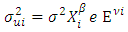 or equivalently
 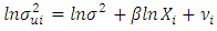 | (2) |
Where  is the stochastic disturbance term. Assuming
  is not known,
  will be used as an estimate of
  and
and  is then obtained by regressing
  on
on  this is given as;
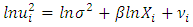 | (3) |
If  is statistically significant, it suggests heteroscedasticity, if otherwise then homoscedasticity is assumed. So Park test is seen as a 2-stage procedure, where
  is obtained from Ordinary Least Square regression disregarding heteroscedasticity and then in the 2nd stage, the regression in equation (3) is done, and the significance of
  is tested.♣ Glejser Test:- This test was developed by Herbert Glejser. [3], suggested estimating the original regression with Ordinary Least square to obtain the residual
  and regressing the absolute value of
  on the explanatory variable that is thought on a priori grounds to be associated with the heteroscedastic variance
  He uses the functional forms;
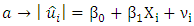 | (4) |
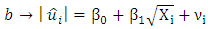 | (5) |
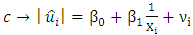 | (6) |
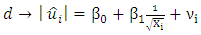 | (7) |
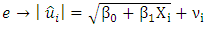 | (8) |
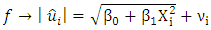 | (9) |
Given that  is the error term. In this work we considered the Glejser functional forms b, c and d, that is equations 5-7.♣ GoldFeld-Quandt Test: This test is applicable for large samples and it assumes that the observations must be at least twice as many as the parameters to be estimated. The test also assumes normality and serial independent error terms. It compares the variance of error terms across discrete subgroups. [5], in their paper they stated that; The power of this test will clearly depend upon the value of the n2, the number of omitted observations and for every large value of
  the power will be small, but it is not obvious that the power increases monotonically as
  They also stated that the power of the test will clearly depend on the nature of the sample values for the variable which is the deflator.♣ Breusch-Pagan Test: This test improves on the limitation of Goldfeld-Quandt test. The basic idea behind this test is the assumption that the heteroscedastic variance
  is a linear function of some nonstochastic variable, say Z, written as;
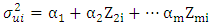 | (10) |
and it is assumed that  Therefore to test whether
  is homoscedastic, one can test the hypothesis that:
 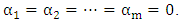 ♣ White’s Test:- [13], proposed a test which is very similar to that of Breusch-Pagan. This test does not rely on normality assumption and it’s very easy to implement. The test is based on the residual of the fitted model. To carry out the test, auxillary regression analysis is used by regressing the squared residual from the original model on a set of original regressors, the cross products of the regressors and the squared regressors. Then the
  from the auxillary regression is then multiplied by n (sample size), giving:
4. Corrective Measures
All the above mentioned tests have some form of strengths and weaknesses, but we will not discuss that in this work. In the event that heteroscedasticity exits and  is known, [6] recommended the adopting of the method of weighted least square, but in instances where
  is not known, he also suggested the use of White’s heteroscedasticity-consistent standard error estimator of ordinary least square parameter estimate as a remedial measure. But with these approaches, the regression model is estimated using the Ordinary Least Square and an alternative method of estimating the standard errors that does not assume homoscedasticity will then be employed, making the work a bit prolonged. [7], recommended that the easiest method is to use some kind of variance stabilizing transformations of Y. Commonly recommended transformations include
 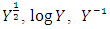 or the Box-Cox transformation. In view of all these, the primary objective is to eliminate heteroscedasticity present in our economic data by employing the Box-Cox transformation as a remedial or corrective measure.
4.1. Box-Cox Transformation
[1], proposed a parametric power transformation technique in order to reduce anomalies such as non-additivity, non-normality and heteroscedasticity. The main aim of Box-Cox transformation is to ensure that the usual assumption for linear model is satisfied. At the core of the Box-Cox transformation is an exponent, lambda (λ), which varies from -5 to 5. All values of λ are considered and the optimal value for your data is selected. The optimal value is the one which results in the best approximation of a normal distribution curve. The transformation of Y has the form;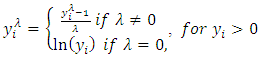 | (11) |
When transforming the dependent variable and trying to find the best value of λ in the Box-Cox transformation, the problem of the scores no longer being in their original metric arises. Consequently the residual sum of squares no longer has the same statistical meaning as it did prior to transformation. This means that the best λ will not be found by comparing the several competing values of λ to the residual sum of squares, [11]. Sakia [11], further stated that this problem was solved by the Box-Cox transformation because it incorporates the geometric mean of the dependent variable Y, denoted a  to simplify the derivation of the maximum-likelihood method. Equation (11) then becomes;
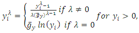 | (12) |
Given that 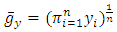 and it follows that
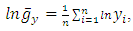 The power parameter λ can be estimated using maximum likelihood estimation to obtain the optimal λ that minimizes the sum of squares of error of the transformed data or maximizes the log-likelihood function from a range of λ values usually in the interval [-2,2] as given in [11].
5. Analysis and Results
5.1. Normality Test
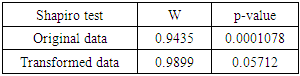
The graphical methods of checking data normality have raised a lot of discussions in the statistical world about the meaning of all the plots and what is seen as normal. Bearing that in mind we decided to apply a formal test that is widely used called the Shapiro-wilks test. Our results are shown below:Table 1. Normality test
 |
| |
|
The transformed data proved to be normally distributed with a p-value = 0.05712.
5.2. Multicollinearity Test
Multicollinearity is a phenomenon in which one predictor variable in a multiple regression model can be linearly predicted from the others with a substantial degree of accuracy. A simple approach to identify multicollinearity in a multiple regression model among explanatory variables is the use of variance inflation factors (VIF). If the VIF is > 10 multicollinearity is strongly suggested but if it is < 10 then it suggests no evidence of multicollinearity. In our analysis the value of the VIF is 3.761295, this suggests that there is no multicollinearity among the explanatory variables.
5.3. Hateroscedasticity Test
Hypothesis: (Homoscedastic)
 (Heteroscedastic)Our regression model is given in equation (1) and below is our estimated model.Our estimated model before Box-Cox transformation is given as;
 | (13) |
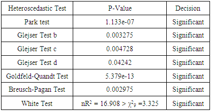
With an R2 = 0.6993, p-value of < 2.2e-16 and an F-statistic of 63.96. The shows the model is significant. Our analysis also showed an AIC of 1667.924 and a BIC of 1684.394.Table 2. Heteroscedastic tests with the P-Values before Box-Cox Transformation
 |
| |
|
Our estimated model after Box-Cox transformation is given as; | (14) |
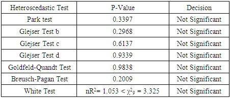
With an R2= 0.7341, p-value of < 2.2e-16 and F-statistics of 75.94, which also shows that the model is significant and the analysis also gave an AIC of -640.6783 and a BIC of -624.2087.Table 3. Heteroscedastic Tests and the P-Values after Box-Cox Transformation
 |
| |
|
6. Discussion
In this work, we made use of an economic data, with Gross Domestic Product (GDP) as the response variable and the independent variables as: Inflation, Trade, Civil-liability and Population. Our estimated model before Box-Cox transformation is found in equation (13). This model gave an R-squared of 0.6993, an AIC of 1667.924 and a BIC of 1684.394. We established the existence of heteroscedasticity through our tests as seen in table 2 that all the tests were found to be significant. A Box-Cox transformation was applied to the response variable, giving us the estimated model in equation (14) which is seen to be significant with a p-value < 2.2e-16 having an R-squared of 0.7341, an AIC of -640.6783 and a BIC of -624.2087. The R-squared and AIC shows that the model after the transformation is a better model compared to the model before the transformation. Our table 3 shows the results of all the tests after Box-Cox transformation have been applied and from the table we can see that all the tests showed a non significant result, proving to us that the problem of varying variance have been remedied by the Box-Cox transformation.
References
| [1] | Box G.E.P and Cox D. R. (1964): An Analysis of Transformation; Journal of Royal Statistics Society, Series B, 26, 211-252. |
| [2] | Buthmann A. (2008): Making Data normal Using Box-Cox Power Transformation, https://www.isixsigma.com. |
| [3] | Glejser H. (1969): A New Test for Heteroscedasticity; Journal of American Statistical Association, 64(235); pp315-323. |
| [4] | Godfrey L. G. (1996): Some Results on the Glejser and Koenker Tests for heteroscedasticity; Journal of Econometrics 72(275). |
| [5] | Gold Feld S. M. and Quandt R.E. (1965): Some Tests of Homoscedasticity; Journal of American Statistical Association; 60(310); pp539-547. |
| [6] | Gujarati D. N. and Porter D. C., (2009): Basic Econometrics, McGraw-Hill Companies Inc. New York, pp389-394. |
| [7] | Hayes A. F. and Cai L. (2007): Using Heteroscedasticity-Consistent Standard Error Estimators in OLS Regression: An Introduction and Software Implementation; Behaviour Research Methods, 39(4), pp 709-722. |
| [8] | Hill R. C., Griffiths W. E. and Lim G.C. (2007): Principles of Econometrics; John Wiley & Sons Inc. New Jersey. |
| [9] | Lyon & Tsai (1996): A Comparison of Tests for Heteroscedasticity; The Statistician, 45, 3, 337-349. |
| [10] | Park R. E. (1966): Estimation with Heteroscedastic Error Terms; Econometrica; 34(4), pp 888. |
| [11] | Sakia R.M. (1992): The Box-Cox Transformation Technique: A Review, The Statistician, 41, pp169-178. |
| [12] | Transformation: An Introduction; fmwww.bc.edu > repec > bocode > transint. Accessed 29th of Nov. 2017. |
| [13] | White H. (1980): A Heteroscedasticity Consistent Covariance Matrix Estimator and A Direct Test for heteroscedasticity; Econometrica; vol 44, pp 817-818. |
| [14] | Wikipedia, Power transform; https://en.m.wikipedia.org. Accessed 29th of Nov, 2017. |

 Abstract
 Reference
 Full-Text PDF
 Full-text HTML