1. Introduction

In probability theory, zero-truncated distributions are certain discrete distributions having support the set of positive integers. Zero-truncated distributions are suitable models for modeling data when the data to be modeled originate from a mechanism which generates data excluding zero counts.

Suppose is the original distribution. Then the zero-truncated version of can be defined as

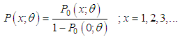(1.1)

The Poisson-Akash distribution (PAD) having probability mass function (pmf)

(1.2)

was introduced by Shanker (2017). Shanker (2017) studied its various statistical properties, estimation of parameter using both the method of moments and the method of maximum likelihood, and applications of PAD to model count data from different fields of knowledge. Shanker et al (2016) has detailed study about the applications of PAD for modeling data from various fields of knowledge. 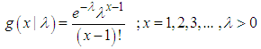The PAD arises from the Poisson distribution when its parameter follows Akash distribution introduced by Shanker (2015) with probability density function (pdf)

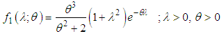(1.3)

Detailed discussion about mathematical and statistical properties, estimation of parameter and applications for modeling lifetime data of Akash distribution has been mentioned in Shanker (2015) and shown that (1.3) is a better model than both exponential and Lindley (1958) distributions for modeling lifetime data from engineering and biomedical sciences.

In this paper, a zero-truncated Poisson-Akash distribution (ZTPAD) has been suggested by taking the zero-truncated version of PAD introduced by Shanker (2017). The moments about origin and moments about mean of ZTPAD have been obtained and thus expressions for coefficient of variation, skewness, kurtosis, and index of dispersion have been given. Estimation of its parameter has been discussed using both the method of moments and the method of maximum likelihood estimation. Finally, applications of ZTPAD to three observed real datasets have been given to test its goodness of fit over zero-truncated Poisson distribution (ZTPD), Zero-truncated Poisson-Lindley distribution (ZTPLD), and zero-truncated Poisson-Sujatha distribution (ZTPSD).

2. Zero-Truncated Poisson-Akash Distribution

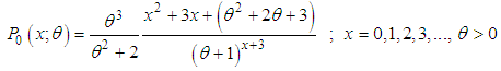
Using (1.1) and (1.2), the pmf of zero-truncated Poisson-Akash distribution (ZTPAD) can be obtained as

(2.1)

The ZTPAD can also be obtained by compounding size-biased Poisson distribution (SBPD) having pmf.

(2.2)

when the parameter of SBPD follows a continuous distribution having pdf

(2.3)

where .

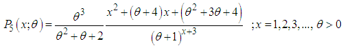
The pmf of ZTPAD is thus obtained as

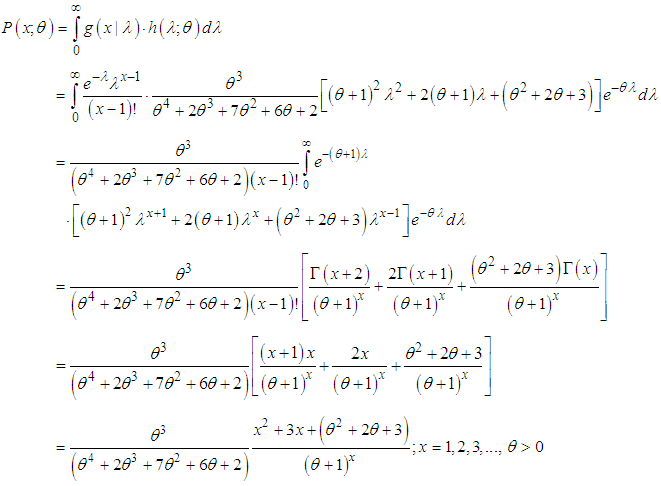(2.4)

which is the pmf of ZTPAD with parameter , obtained earlier in (2.1). The main reason for finding the pmf of ZTPAD as a mixture of SBPD with an assumed continuous distribution (2.3) is to obtain the moments easily. The graph of the pmf of ZTPAD for varying values of the parameter has been shown in figure 1. The graphs show that the pmf is monotonically decreasing for increasing values of the parameter .

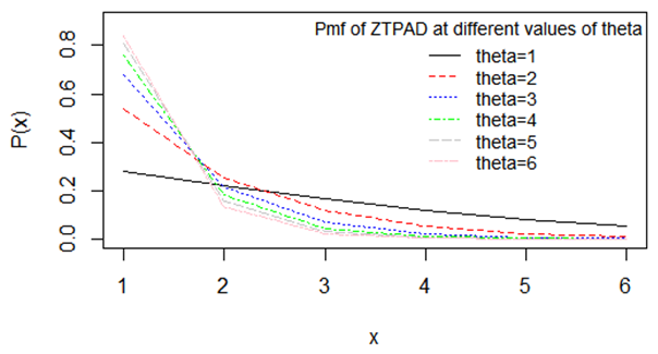Figure 1. Graphs of the pmf of ZTPAD for varying values of the parameter θ

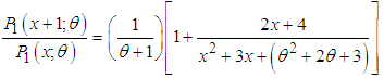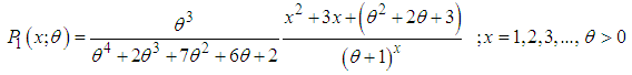
Since is a decreasing function of x, is log-concave. Therefore, ZTPAD is unimodal, has increasing failure rate (IFR), and hence increasing failure rate average (IFRA). It is new better than used (NBU), new better than used in expectation (NBUE), and has decreasing mean residual life (DMRL). Detailed discussions and interrelationships between these aging concepts are available in Barlow and Proschan (1981).

Recall that the pmf of zero-truncated Poisson- Lindley distribution (ZTPLD) given by

(2.5)

has been introduced by Ghitany et al (2008 b). The pmf of Poisson-Lindley distribution (PLD) given by

(2.6)

has been obtained by Sankaran (1970) by compounding Poisson distribution with Lindley distribution, introduced by Lindley (1958) having pdf

(2.7)

Ghitany et al (2008 a) have detailed study about various properties, estimation of parameter and the application of Lindley distribution for modeling waiting time data in a bank. Shanker et al (2015 a) have detailed and critical study on modeling of lifetimes data using both exponential and Lindley distribution and observed that there are many examples where exponential distribution gives better fit than the Lindley distribution. Shanker and Hagos (2015 a) have discussed the applications of PLD for modeling data from biological sciences. Shanker et al (2015 b) have done extensive study on the comparison of ZTPD and ZTPLD with respect to their applications in datasets excluding zero-counts and showed that in demography and biological sciences ZTPLD gives better fit than ZTPD while in social sciences ZTPD gives better fit than ZTPLD.

Note that the pmf of zero-truncated Poisson-Sujatha distribution (ZTPSD) given by

(2.8)

has been introduced by Shanker and Hagos (2015 b) for modeling count data excluding zero counts from different fields of knowledge. Various interesting properties, estimation of parameter and applications of ZTPSD have been mentioned in Shanker and Hagos (2015 b).

Shanker (2016 b) has obtained the Poisson-Sujatha distribution (PSD) having pmf

(2.9)

Shanker (2016 b) obtained the PSD as a Poisson mixture of Sujatha distribution when the parameter of the Poisson distribution follows Sujatha distribution, introduced by Shanker (2016 a) having pdf

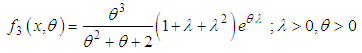(2.10)

Shanker (2016 a) has detailed study about various mathematical and statistical properties, estimation of parameter and applications of Sujatha distribution for modeling lifetime data from biomedical science and engineering and it has been observed that Sujatha distribution is a better model than both exponential and Lindley (1958) distributions. Shanker and Hagos (2016 b) have discussed applications of PSD to model data from ecology and genetics and observed that PSD is a better model than both the Poisson and Poisson-Lindley distributions. Shanker and Hagos (2016 c) have studied comparative study on ZTPD, ZTPLD and ZTPSD for modeling data from biological science, demography and thunderstorms.

3. Moments

The rth factorial moment about origin of ZTPAD (2.1) can be obtained as

Using (2.4), we have

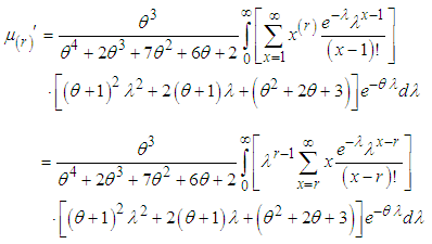Taking , we get

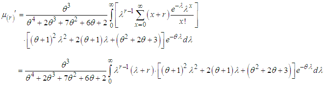Using gamma integral and a little algebraic simplification, we get the expression for the rth factorial moment about origin of ZTPAD as

(3.1)

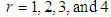Substituting in equation (3.1), the first four factorial moments about origin can be obtained and using the relationship between moments about origin and factorial moments about origin, the first four moments about origin of ZTPAD can be obtained as

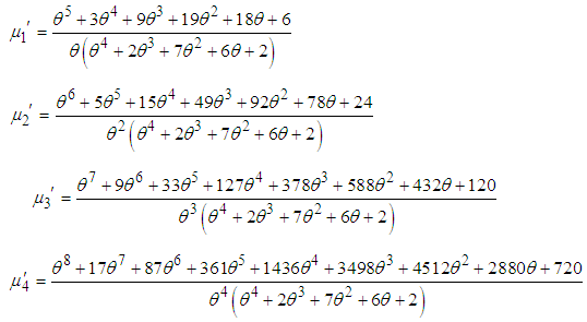Again using the relationship between moments about origin and central moments, the central moments of ZTPAD are thus obtained as

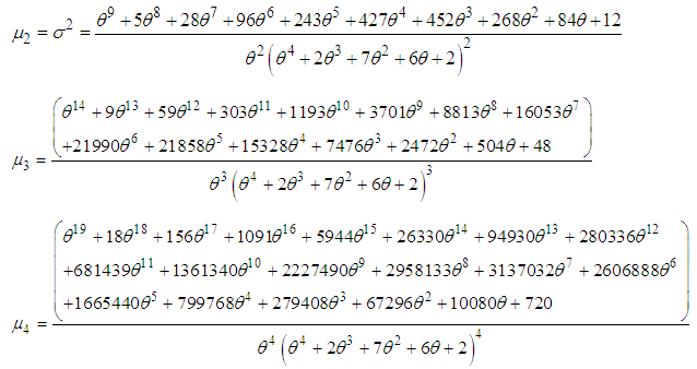Finally, the coefficient of variation (C.V), coefficient of Skewness , coefficient of Kurtosis , and index of dispersion of ZTPAD are obtained as

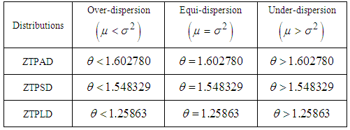
The condition under which ZTPAD is over-dispersed , equi-dispersed , and under-dispersed are presented in table 1 along with ZTPSD and ZTPLD.

Table 1. Over-dispersion, equi-dispersion and under-dispersion of ZTPAD, ZTPSD and ZTPLD

The nature and behavior of coefficient of variation, coefficient of skewness, coefficient of kurtosis, and index of dispersion of ZTPAD for varying values of the parameter are shown in figure 2. It is obvious that the coefficient of variation and the index of dispersion are monotonically decreasing while the coefficient of skewness and coefficient of kurtosis are monotonically increasing for increasing values of the parameter .

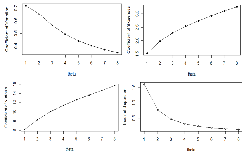Figure 2. Graphs of coefficient of variation, coefficient of skewness, coefficient of kurtosis, and index of dispersion of ZTPAD for varying values of the parameter θ

4. Estimation of Parameter

4.1. Method of Moment Estimate (MOME)

Let be a random sample of size n from the ZTPAD (2.1). Equating the population mean to the corresponding sample mean, the MOME of is the solution of the following non-linear equation

where is the sample mean.

4.2. Maximum Likelihood Estimate (MLE)

Let be a random sample of size n from the ZTPAD (2.1) and let be the observed frequency in the sample corresponding to such that , where k is the largest observed value having non-zero frequency. The likelihood function L of the ZTPAD is given by

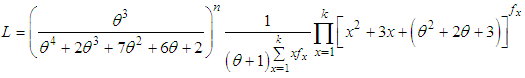The log likelihood function is given by

and the log likelihood equation is thus obtained as

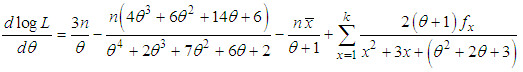The maximum likelihood estimate of is the solution of the equation and is given by the solution of the following non-linear equation

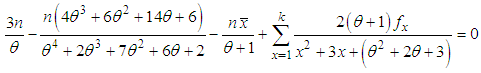where is the sample mean. This non-linear equation can be solved by any numerical iteration methods such as Newton- Raphson method, Bisection method, Regula –Falsi method etc. In this paper Newton-Raphson method has been used to solve the above non-linear equation to estimate the parameter. The initial value of the parameter has been taken from the MOME estimate of the parameter.

5. Applications

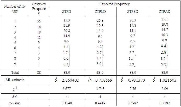
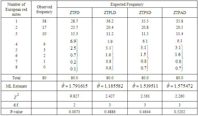
The ZTPAD has been fitted to a number of real datasets to test its goodness of fit over ZTPD, ZTPLD and ZTPSD and it has been observed that in most cases it gives better fit. Maximum likelihood estimate of the parameter has been used to fit ZTPD, ZTPLD, ZTPSD, and ZTPAD. Here three examples of real datasets have been presented. The dataset in table 2 is the data regarding the number of counts of flower heads as per the number of fly eggs reported by Finney and Varley (1955), the dataset in table 3 is the data regarding the number of snowshoe hares counts captured over 7 days reported by Keith and Meslow (1968) and the dataset in table 4 is the data regarding the number of European red mites on apple leaves reported by Garman (1923).

It is obvious from the values of Chi-square and p-value that ZTPAD gives much closer fit than ZTPD, ZTPLD and ZTPSD. Therefore, ZTPAD can be considered as an important tool for modeling count data excluding zero-count over ZTPD, ZTPLD and ZTPSD.

The fitted plots of ZTPD, ZTPLD, ZTPSD and ZTPAD for datasets in tables 2, 3, and 4 have been shown in figure 3 and it is also obvious that ZTPAD gives closer fit in all datasets.

Table 2. The numbers of counts of flower heads as per the number of fly eggs reported by Finney and Varley (1955)

Table 3. The number of snowshoe hares counts captured over 7 days, reported by Keith and Meslow (1968)

Table 4. Number of European red mites on apple leaves, reported by Garman (1923)

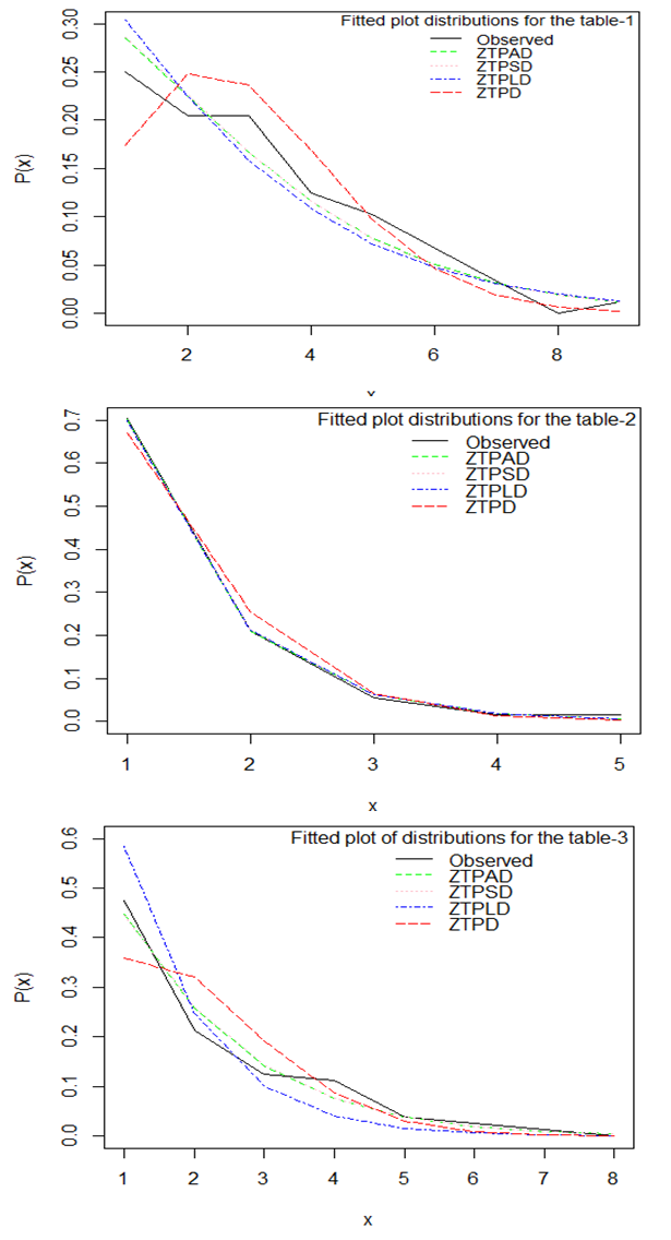Figure 3. Fitted plots of ZTPD, ZTPLD, ZTPSD and ZTPAD for datasets in tables 2, 3, and 4

6. Concluding Remarks

A zero-truncated Poisson-Akash distribution (ZTPAD) has been introduced. The general expression for the rth factorial moment about origin has been obtained and thus its raw moments and central moments have been given. The coefficients of variation, skewness, kurtosis, and the index of dispersion of ZTPAD have been obtained. The method of moments and the method of maximum likelihood estimation have been discussed for estimating the parameter of ZTPAD. The goodness of fit of ZTPAD has been discussed with three examples of real datasets and the fit has been compared with ZTPD, ZTPLD and ZTPSD and the fit by ZTPAD has been found to be quite satisfactory. Therefore, ZTPAD can be considered one of the important distributions to model count datasets which structurally excludes zero counts.

ACKNOWLEDGEMENTS

Author is grateful to the Editor-In-Chief and the anonymous reviewer for fruitful comments on the paper which improved the presentation of the paper.