1. Introduction

Classical statistical procedures are designed in such a way that they can produce best result when underlying assumptions on the data’s population distributions are true. But in practice, we often have to deal with the situation when actual situations depart from the ideal situation described by such assumptions, and it has been proved that the performance of many statistical techniques suffers badly when the real situation departs from ideal situation. The performance of ANOVA test also suffers badly when the validity of normality assumption does not hold. Generally the extent of deviation from normality is an important factor that supervises the strength (weakness) of the ANOVA procedure. The main concern of this study is to observe the performance of conventional ANOVA test under various nonnormal situations for multiple linear regression models. Simultaneous measure of the skewness and kurtosis parameter has been considered as the measure of extent of non-normality. The skewness parameter measure the degree of distortion or deviation from normality and the kurtosis measures the peakedness or thickness of the tail of the distribution. In this manuscript, the simplest possible multiple linear regression model i.e. three variable multiple regression model with one dependen t variable and two explanatory variable is considered and the extent of effect of deviation from normality is measured by considering the model error from g-and-k distribution.

A number of studies on robustness and tests of normality shows many contributions from the most outstanding theorists and practitioners of statistics. The effect of non-normality on the power of analysis of variance test has been studied by Srivastava (1959) by investigating the non-central distribution of the variance ratio. Box and Watson (1962) demonstrated the overriding influence which the numerical values of regression variables have in deciding sensitivity to non-normality and also showed the essential nature of this dependency. Tiku (1971) calculated the values of the power of the F test employed in analysis of variance under non-normal situations and compared with normal- theory values of the power. Kanji (1976) discussed about simulation methods for calculating power values in the case of non-normal errors. He used Erlangian and contaminated normal distribution as an example of non-normal error distribution. MacGillivray and Balanda (1988) studied on skewness and kurtosis, and considered the concept of anti-skewness to use it as a tool to discuss the idea of kurtosis in asymmetric univariate distributions. Mukhter and Shubhas (1996) investigated the robustness to nonnormality of the null distribution of the standard F-tests for regression coefficients in linear regression models. Assuming the errors to be nonnormal with finite moments, the null distribution of the F-statistic is derived. Khan and Rayner (2001) made an attempt to study the effects of the strong assumptions required for ANOVA and also investigated the effects of the departure from the normality of error on the power function by using g-and-k distribution. Khan and Rayner (2003) investigated the effect of deviation from the normal distribution assumption by considering the power of two many –sample location test procedure: ANOVA (parametric) and Kruskal-Walis (non-parametric). Rasch and Gulard (2004) presented some results of a systematic research of robustness of statistical procedures against non-normality. Serlin and Harwell (2004) observed some more powerful tests of predictor subsets in regression analysis under non-normality. A Monte Carlo study of tests of predictor subsets in multiple regression analysis indicates that various nonparametric tests show greater power than the F test for skewed and heavy-tailed data. These nonparametric tests can be computed with available software. (PsycINFO Database Record (c) 2012 APA, all rights reserved).

Yanagihara (2007) presented the conditions for robustness to non-normality on three test statistics for a general multivariate linear hypothesis, which were proposed under the normal assumption in a generalized multivariate analysis of variance (GMANOVA). Mortaza et al. (2007) provided a study on partial F-test for multiple linear regression models. They showed a power comparisons between the partial F tests and new test to assess when the new tests are more or less powerful than the partial F tests.

Schmider et al (2010) provided empirical evidence to the robustness of the analysis of variance (ANOVA) concerning violation of the normality assumption is presented by means of Monte Carlo methods. Khan and Hossain (2010) suggested a numerical likelihood ratio test for testing the location equality of several populations under quantile function distribution approach. Lantz B. (2012) investigated the relationship between population non-normality and sample non-normality with respect to the performance of the ANOVA, Brown-Forsythe test, Welch test, and Kruskal-Wallis test when used with different distributions, sample sizes, and effect sizes. The overall conclusion is that the Kruskal-Wallis test is considerably less sensitive to the degree of sample normality when populations are distinctly non-normal and should therefore be the primary tool used to compare locations when it is known that populations are not at least approximately normal. Jahan and khan (2012) demonstrated the extent of effect of non-normality on power of the t-test for simple linear regression model using g-and-k distribution.

It is clear that a wide range of studies have been made on the non-normality of the model error but so far no studies has been conducted to see what extent of deviations from normality causes what extent of effect on the size and power of ANOVA-test for multiple linear regression model. This paper contains a power curve study to examine the extent of effect on size and power of ANOVA test for multiple linear regression models with two explanatory variables on a wide variety of normal and non-normal situation and for different sample sizes. The power of ANOVA test for multiple linear regression models is measured numerically and shown graphically.

2. Multiple Linear Regression Model

The Three -Variable Model

The multiple linear regression models with two explanatory variables can be written as follows:

(2.1)

Where, is the dependent variable, and are explanatory variables, is the stochastic disturbance term, and 𝑖 is the 𝑖th observation. is the intercept term, it gives the mean or average effect on of all the variable excluded from the model, although its mechanical interpretation is the average value of when and are set equal to zero. The coefficients and are called partial regression coefficients. measures the change in the mean value of per unit change in , holding the value of constant. Likewise, measures the change in the mean value of per unit change in , holding the value of constant. The coefficients and are called partial regression coefficients. measures the change in the mean value of per unit change in holding the value of constant.

3. The g-and-k Distribution

The g-and-k distribution (MacGilivray and Canon) can be defined in terms of its quantile function as:

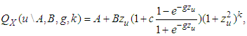(3.1)

Where, and >0 are the location and scale parameters respectively, measures skewness in the distribution, measures kurtosis (in general sense of peakness/tailedness) in the distribution and is the th quantile of a standard normal variate, and is a constant chosen to help produce proper distributions. It can be clearly observed that for , the quantile function in (3.1) is just the quantile function of a standard normal variate.

The sign of the skewness parameter indicates the direction of skewness; indicates the distribution is skewed to the left, and indicates skewness to the right. Increasing/decreasing the unsigned value of increases/decreases the skewness in the indicated direction. When the distribution is symmetric.

The kurtosis parameter , for the -and- distribution, behaves similarly.

Increasing increases the level of kurtosis and vice versa. The value corresponds to no extra kurtosis added to the standard normal base distribution. However, this distribution can represent less kurtosis than the normal distribution, as can negative values. If curves with more kurtosis required then base distribution with less kurtosis than standardized normal distribution can be used. For these distributions is the value of overall (MacGilivray). For an arbitrary distribution, theoretically the overall asymmetry can be as large as one, so it would appear that for , data or distribution could occur with skewness that cannot be matched by these distributions. However for , the larger the value chosen for , the more restrictions on are required to produce a completely proper distribution. Real data seldom produce overall asymmetry values greater than 0.8 (MacGilivray and Canon). The value of is taken as 0.83 throughout this paper. To examine extent of the effect of different level of non-normality on the test of multiple linear regression models, it is considered that the random error belongs to the -and- distribution.

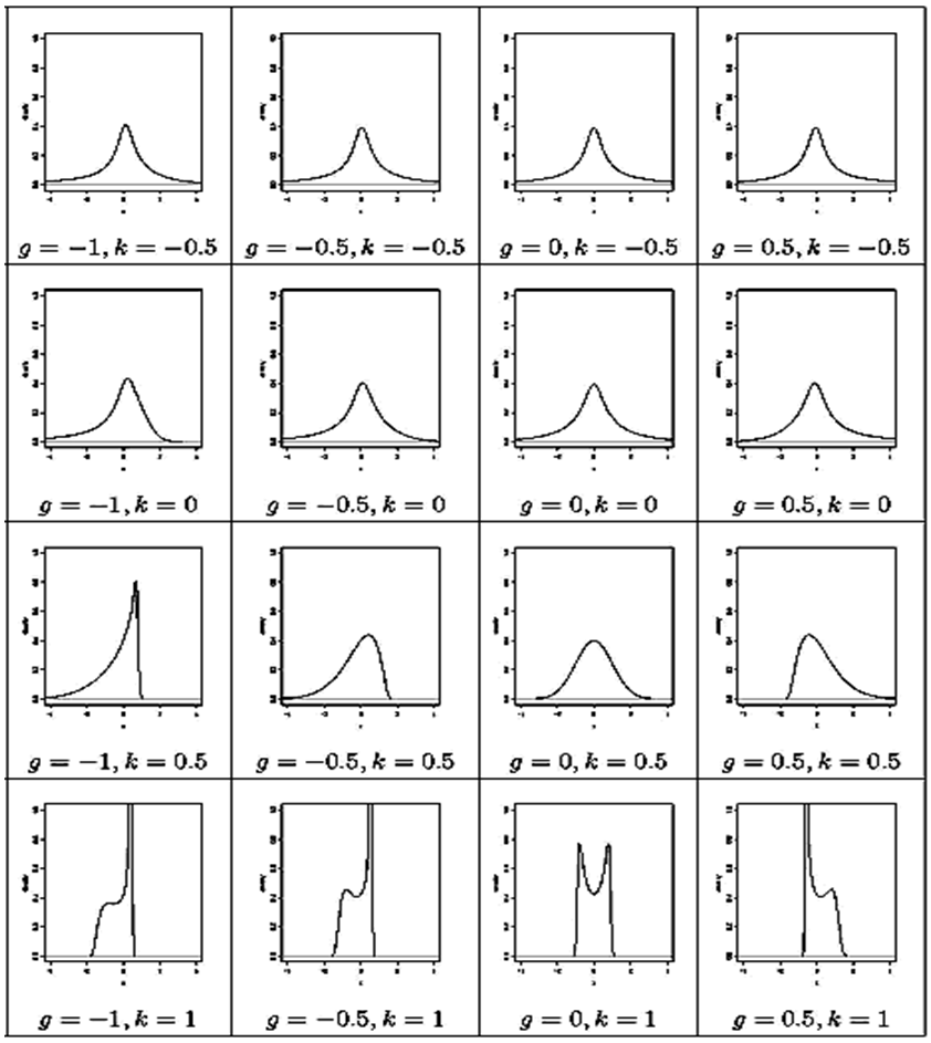Figure 1. Density curves of g-and-k distribution for different combination of g and k

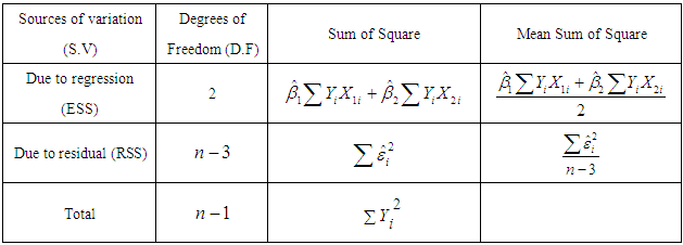
4. The Analysis of Variance Approach for Testing the overall Significance of an observed Multiple Regression: The F -test

Analysis of variance (ANOVA) is a popular and widely used technique in the field of statistics. Besides being the appropriate procedure for testing the equality of several means, the ANOVA has a much wider applications. The objective of the ANOVA procedure lie mainly in estimating and testing hypotheses about the treatment effect parameters. The usual 𝑡 test cannot be used to test the joint hypothesis that the true partial slope coefficients are zero simultaneously. However this joint hypothesis can be tested by the analysis of variance technique which can be demonstrated as follows:

Table 1. ANOVA table for the Three-variable regression

Now under the assumption of normal distribution for and for the null hypothesis

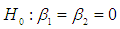
At least one is not equal to zero; 𝑖 = 1,2.

Then the test statistic

(4.1)

is distributed as the distribution with 2 and df. Therefore, the value of (4.1) provides a test of null hypothesis that the true slope coefficients are simultaneously zero. The null hypothesis can be rejected if the value computed from (4.1) exceeds the critical value from the table at percent level of significance, otherwise cannot be rejected.

5. Simulation Study

In this paper, multiple linear regression models with two explanatory variables is considered. As it is known that the error term of multiple linear regression models are normally distributed but here in this paper, the random error term is assumed to follow the g-and-k distribution. The extent of non-normality on the size and power of ANOVA test is observed by varying the skewness and the kurtosis parameter of the -and distribution. Using the g –and -k distribution allows us to quantify how much the data depart from normality in terms of the values chosen for the g (skewness) and k (kurtosis) parameters. For g = k = 0, the quantile function for and distribution is just the quantile function of a normal variate.

To observe the power of the tests, expression for the power curve is required. However, in practice, to obtain analytic expressions for these power functions is impractical. Instead, a simulation is conducted to estimate these power function for various combinations of the g and k parameter values for the error distribution from the and distribution. While simulating for the test, A is taken to be the location which is the median in case of and distribution but for non-normal situations the mean of the distribution moves away from A which actually is the median of the distribution. This departure varies as the values g and k of vary. The values of g and k are taken as and and 1. At first, the effect of non-normality on the size of the F test is observed. For simulating the size of F - test the explanatory variables and are generated from uniform distribution and the random error from g-and-k distribution with location and scale parameters A=0 and B=1, respectively. Using statistical software R data are generated for sample size 20, 30 and 100, and the following hypothesis is tested.

Against the alternative At least one is not equal to zero; 𝑖 = 1,2.

To determine the size of the test, data are generated under the null hypothesis and the test is repeated 5,000 times. The total number of times the hypothesis is rejected is divided by 5,000; tests are carried out using 2.5 percent level of significance.

To compute the power of the F test, the explanatory variables and are considered from uniform distribution and the random error from g-and-k distribution with location parameter A = 0 and scale parameter B = 1. The value of c is considered as 0.83.

To simulate power, the following hypothesis is tested

Against the alternative At least one is not equal to zero; 𝑖 = 1,2.

Data are generated using (-2,-1.5,-1,-.5,0,.5,1,1.5,2) and (-2,-1.5,-1,-.5,0,.5,1,1.5,2) and the test procedures are repeated 5000 times for each pair of (-2,-2),(-2,-1.5), ……………(2,1.5),(2,2). Firstly the number of rejections of the test out of the 5000 times is determined for each pair of in the mentioned set and the total number of rejections are divided by 5000, with the level of significance

6. Size of F-test

First, the effect of non-normality on the size of the F test is considered. For simulating the size of F - test the explanatory variables and is generated from the uniform distribution and the random error from g- and -k distribution with location and scale parameters A = 0 and B =1, respectively. Data are generated for sample size 20, 30 and 100 using statistical software R and the following hypothesis is tested:

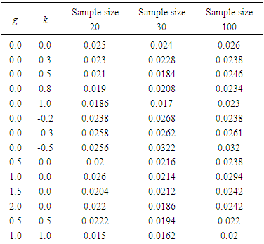
Against the alternative At least one is not equal to zero; 𝑖 = 1,2.

To determine the size of the test, data are generated under the null hypothesis and repeat the test 5,000 times and divide the total number of times the hypothesis is rejected by 5,000; tests are carried out using 2.5 percent level of significance. The size of ANOVA for different combinations of (g, k) are presented in Table 2.

Table 2. Size of ANOVA for different combinations of (g, k) with varying sample sizes

In table 2, some simulation results are presented to see the effect of different level of non-normality on the size of F-test. F-test is size robust under normal situation, but under non-normal situation there is a little effect on the size of the test. For sample size 20 and 30, it is seen that skewness parameter has a very little effect and the kurtosis parameter has moderate effect on the size of F-test. For sample size 100, even in the case of non-normal situation, F -test is almost size robust.

7. Power of F-test

To compute the power of the F test, firstly the explanatory variables and are generated from the uniform distribution and the random error is considered from g-and-k distribution with location parameter A = 0 and scale parameter B =1. The value of c is taken to be 0.83 throughout the paper. To simulate power, the following hypothesis is considered

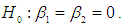
At least one is not equal to zero; 𝑖 = 1, 2.

To see how the power differs as the values of g and k change, the power for specified values of g and k is plotted to get the power curve for ANOVA test with sample sizes n= 20, 30 and 100. To get smooth power curve, many points for different combinations of g and k are used. For each combination we get power. The process is repeated where for each point 5,000 simulations are run.

Figure (2) through (7) shows the power curves for different combination of (g,k) for sample size n = 20, 30 and 100.

8. Discussion of Results

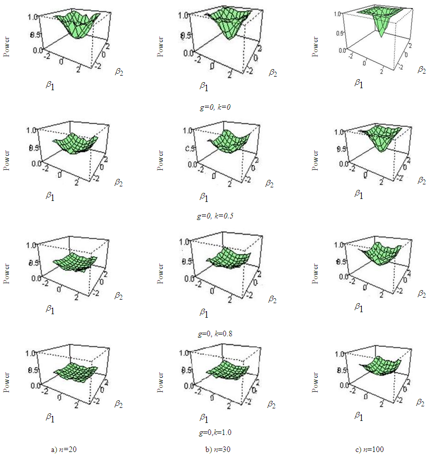
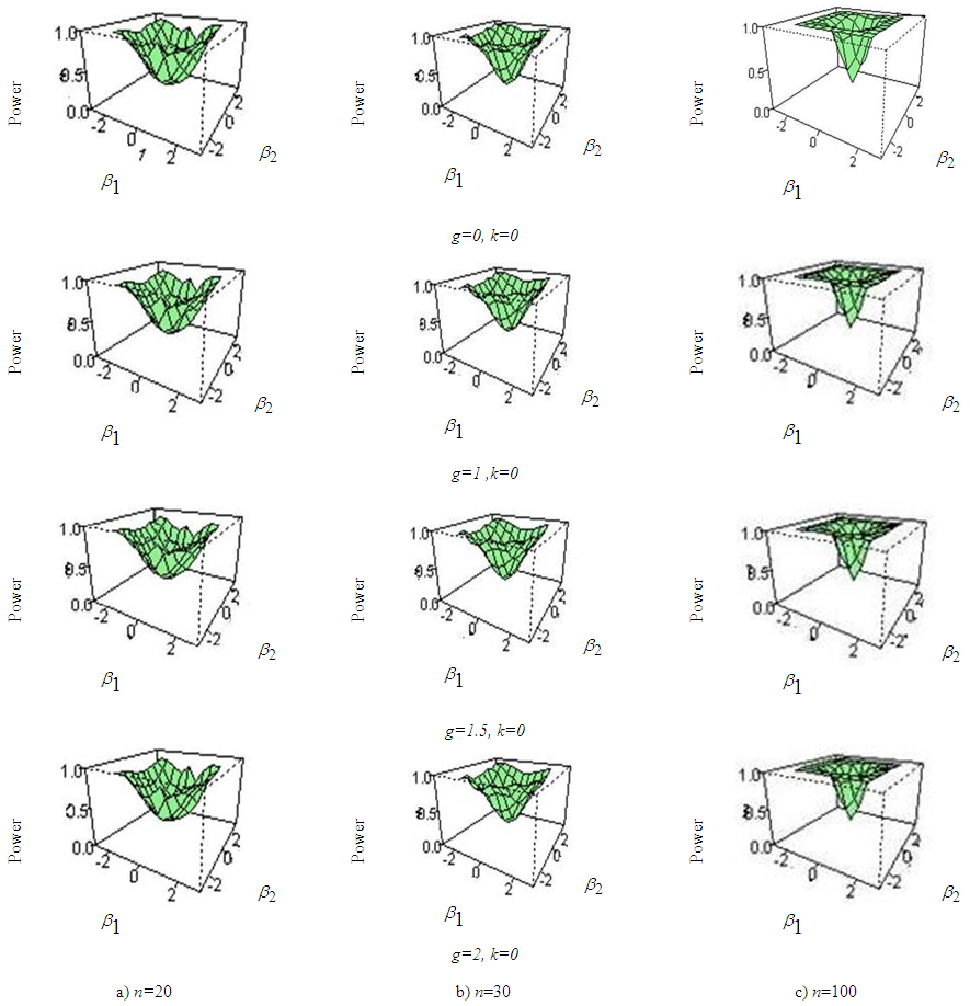
From the figure (2) to figure (7) it is seen that the powers of the test is badly affected by the sample size and kurtosis parameter. The simulation results can be summarized in the following ways:

i) In figure 2, the skewness parameter is considered to be fixed at g=0 but the kurtosis parameter is varied from k=0 to k=1. It is apparent that as the kurtosis parameter increases in positive direction power of the test is vastly decreased than that of normal data. The effect of sample size on the power of the test is also observed in this paper. It is found that the rate of decreasing power in presence of excess kurtosis for small sample (n=20, 30) is higher than that of larger sample size say n=100.

ii) In figure 3, the kurtosis parameter is fixed at k=0 but the skewness parameter is varied from g=0 to g=2. It is examined that power of the test has not much effect when the skewness parameter is varied in positive direction. As the sample size increases power of the test seems to almost robust although the skewness parameter is increased.

iii) In figure 4 and 5, the combination of (g=0, k=0), (g=1, k=0), (g=0, k=1), (g=1, k=1) for sample size 20 and 30 is considered and it is noticed that varying the kurtosis parameter in positive direction has more effect in decreasing the power than that of varying the skewness parameter.

iv) In figure 6 and 7, the effect of increasing the kurtosis parameter in negative direction is observed. The combination of (g=0, k=0), (g=0, k=-.3), (g=0, k=-.5) for sample size 20 and 30 is shown. At first glance it may seems that varying the kurtosis parameter in negative direction gives better power but if a close attention is given at the size of the test it is clearly seen that the size of the test is increased.

v) From figure 2 to 7, it is apparent that the power of ANOVA test is decreased more for small sample size (n=20, 30) than that of large sample size (n=100) under non-normal situation.

Figure 2. Power curve of ANOVA for fixed value of g and varying Kurtosis parameter for (a) sample size n=20, (b) sample size n=30, (c) sample size n=100

Figure 3. Power curve of ANOVA for fixed value of kurtosis and varying skewness parameter for (a) sample size n=20, (b) sample size n=30, (c) sample size n=100

Figure 4. Power curves of ANOVA for a) g=0, k=0, b) g=1,k=0, c)g=0,k=1, d) g=1, k=1 for sample size 20

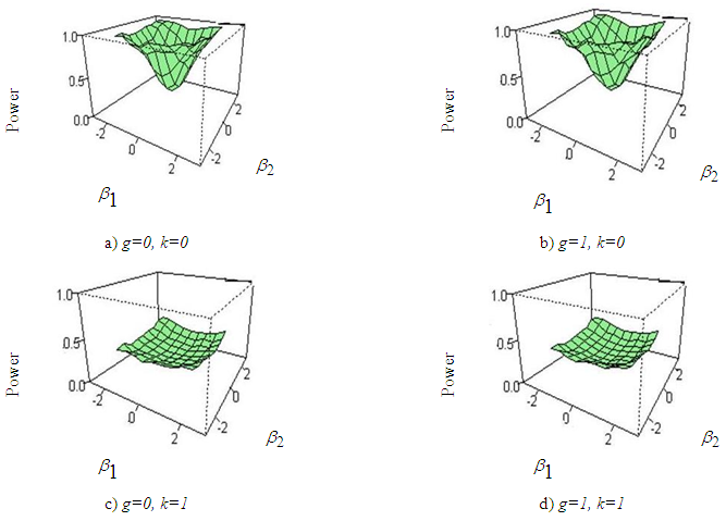Figure 5. Power curves of ANOVA for a) g=0, k=0, b) g=1,k=0, c)g=0,k=1, d) g=1, k=1 for sample size 30

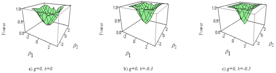Figure 6. Power curves of ANOVA for a) g=0, k=0,b) g=0, k=-0.3, c) g=0, k=-0.5 for sample size 20

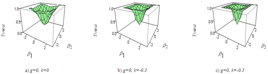Figure 7. Power curves of ANOVA for a) g=0, k=0, b) g=0, k=-0.3, c) g=0, k=-0.5 for sample size 30

9. A Real Life Example (Wolf River Pollution data)

In real life applications, sometimes it may happen that the data do not follow the normal distribution. The examiner needs to identify the amount of deviation from normality and take necessary action to minimize the nonstandard conditions. Khan and Hossain (2010) examined the wolf River Pollution data to investigate how the ANOVA and Kruskal Wallis test perform. Their focus was on hexachlorobenzene (HCB) concentration data (in nanograms per liter) that came out with some features of non-normality. The ANOVA test was carried out for testing the equality of average HCB concentration for different depth although the assumptions were not fully satisfied. The ANOVA test did not provide any strong evidence for the hypothesis that the average HCB concentration for different depths are different, producing a p-value of 0.65. The Kruskal Wallis test produces almost similar p-value of 0.064 like ANOVA. Khan and Hossain (2010) also fitted the data with g-and-k distribution to test whether the data lack normality. MLE was used to estimate the distribution parameters A,B,g, and k to identify the amount of deviation from normality in terms of skewness and kurtosis. The estimated value of and presented the data to be slightly suffered from asymmetry and light tailedness.

10. Conclusions

From the above discussion, the following concluding remarks can be made:

i) As the kurtosis parameter increases in positive direction Power of ANOVA test for multiple linear regression model decreases immensely than that of the normal data.

ii) The skewness parameter seems to have not much effect on the power of ANOVA under non normal situation.

iii) Kurtosis Parameter has more effect in decreasing power of ANOVA test than that of the skewness parameter under non normal situation.

iv) Small sample sizes have more effect in reducing power than that of large sample sizes under non-normal situation.

v) Negative kurtosis gives better power and increases the size of the test.