-
Paper Information
- Paper Submission
-
Journal Information
- About This Journal
- Editorial Board
- Current Issue
- Archive
- Author Guidelines
- Contact Us
American Journal of Mathematics and Statistics
p-ISSN: 2162-948X e-ISSN: 2162-8475
2017; 7(3): 99-107
doi:10.5923/j.ajms.20170703.02

On Size- Biased Two Parameter Poisson-Lindley Distribution and Its Applications
 Abstract
 Reference
 Full-Text PDF
 Full-text HTML
1Department of Statistics, Eritrea Institute of Technology, Asmara, Eritrea
2Department of Statistics, Patna University, Patna, India
Correspondence to: Rama Shanker, Department of Statistics, Eritrea Institute of Technology, Asmara, Eritrea.
| Email: |  |
Copyright © 2017 Scientific & Academic Publishing. All Rights Reserved.
This work is licensed under the Creative Commons Attribution International License (CC BY).
http://creativecommons.org/licenses/by/4.0/

A size - biased version of the two parameter Poisson- Lindley distribution introduced by Shanker and Mishra (2014) has been proposed of which the Ghitany and Al Mutairi’s (2008) size - biased one parameter Poisson-Lindley distribution is a particular case. A general expression for its rth factorial moment about origin has been derived and hence its raw moments and central moments are obtained. The expressions for its coefficient of variation, skewness, kurtosis and index of dispersion have also been given. The method of maximum likelihood and the method of moments for the estimation of its parameters have been discussed. The applications and the goodness of fit of the proposed distribution have been discussed with three data sets excluding zero counts and the fit has been compared with that of size-biased Poisson and size-biased Poisson-Lindley distributions.
Keywords: Size-biased distributions, Two-parameter Poisson-Lindley distribution, Poisson-Lindley distribution, Size-biased distributions, Moments, Estimation of Parameters, Goodness of fit
Cite this paper: Rama Shanker, A. Mishra, On Size- Biased Two Parameter Poisson-Lindley Distribution and Its Applications, American Journal of Mathematics and Statistics, Vol. 7 No. 3, 2017, pp. 99-107. doi: 10.5923/j.ajms.20170703.02.
Article Outline
1. Introduction
- The size - biased distributions arise when the observations generated from a random process do not have equal probability of being recorded and are recorded according to some weight function. When the sampling mechanism is such that the sample units are selected with probability proportional to some measure of the unit size, the resulting distribution is called ‘size-biased distribution’. Fisher (1934) first introduced such distributions to model ascertainment bias and Rao (1965) formulated these in a unifying theory. Patil and Ord (1975) studied the size-biased sampling and the related form-invariant weighted distribution whereas Van Deusen (1986) arrived at size - biased distribution theory independently and applied it to fitting distributions of diameter at breast height (DBH) data arising from horizontal point sampling (HPS). Later, Lappi and Bailey (1987) analyzed HPS diameter increment data using size- biased distribution. Patil and Rao (1977, 1978) examined some general models leading to size - biased distributions. The results were applied to the analysis of data relating to human populations and wild life management. Gove (2003) reviewed some of the recent results on size- biased distributions pertaining to parameter estimation in forestry with special emphasis on Weibull distribution. Simoj and Maya (2006) introduced some fundamental relationships between weighted and unique variables in the context of maintainability function and inverted repair rate. Mir and Ahmad (2009), Das and Roy (2011) and Ducey and Gove (2015) have also studied the various aspects of size - biased distributions.A simple size-biased version of a distribution
 is given by its probability function
 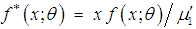 where
where  is the mean of the distribution. Ghitany and Al Mutairi (2008) obtained a size-biased Poisson-Lindley distribution (SBPLD) given by its probability mass function (p.m.f.)
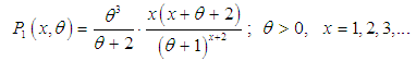 | (1.1) |
 | (1.2) |
 | (1.3) |
 | (1.4) |
 | (1.5) |
 | (1.6) |
 | (1.7) |
 | (1.8) |
 | (1.9) |
 | (1.10) |
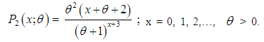
 . Shanker and Mishra (2014) have shown that (1.9) is a better model than the PLD of Sankaran (1970) for analyzing different types of count data. This distribution arises from the Poisson distribution when its parameter
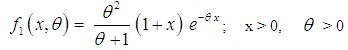
  follows the Shanker and Mishra (2013) two parameter Lindley distribution having probability density function (p.d.f)
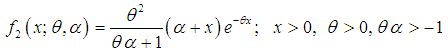 | (1.11) |
2. A Size- Biased Two Parameter Poisson-Lindley Distribution
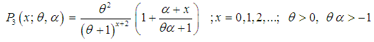
- A size -biased version of the two parameter Poisson-Lindley distribution (SBTPPLD) with parameters
 and
and  can be obtained as
 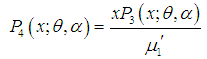 | (2.1) |
 from (1.9) and
  from (1.10), we get
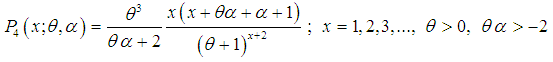 | (2.2) |
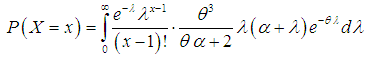
 , SBTPPLD (2.2) reduces to SBPLD (1.1). The SBTPPLD (2.2) can also be obtained from the size- biased Poisson distribution when its parameter
  follows a size-biased two parameter Lindley distribution of Shanker and Mishra (2013) with p.d.f.
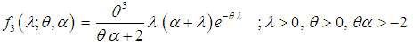 | (2.3) |
 | (2.4) |
 | (2.5) |
 | (2.6) |
 ,
,  is log-concave. This implies that the SBTPPLD is unimodal, has an increasing failure rate (IFR) and so increasing failure rate average (IFRA). It is new better than used (NBU), new better than used in expectation (NBUE) and has decreasing mean residual life (DMRL). Details about the definitions and relationship of these aging concepts can be seen in Barlow and Proschan (1981).
3. Moments and Related Measures
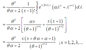
- The rth factorial moment about origin of the SBTPPLD (2.2) can be obtained as
 From (2.4), we get
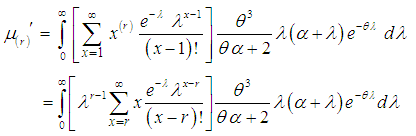 Taking
  in place of
  , we get
 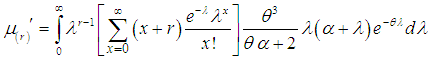 Clearly the expression within the bracket is
  and hence we have
 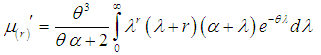 Using gamma integral and a little algebraic simplification, a general expression for the rth factorial moment about origin of SBTPPLD is obtained as
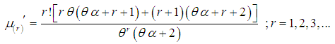 | (3.1) |
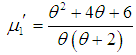
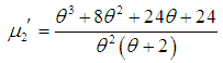
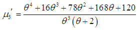
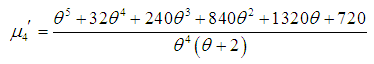
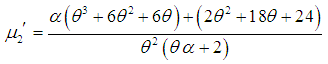
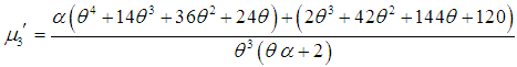
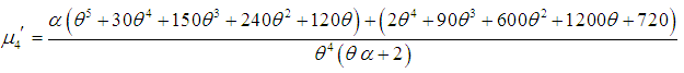
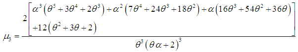
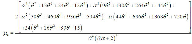
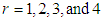 in (3.1), the first four factorial moments about origin can be obtained and then using the relationship between factorial moments and moments about origin, the first four moments about origin of SBTPPLD are obtained as
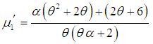 | (3.2) |
 | (3.3) |
 | (3.4) |
 | (3.5) |
 | (3.6) |
 | (3.7) |
 | (3.8) |
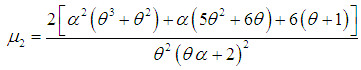
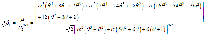
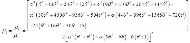
 , coefficient of skewness
 , coefficient of kurtosis
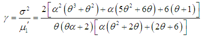
 and index of dispersion
  of SBTPPLD are thus given by
 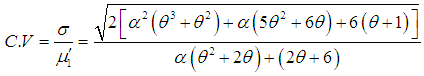 | (3.9) |
 | (3.10) |
 | (3.11) |
 | (3.12) |
 these expressions reduce to the respective expressions of the SBPLD (1.1).
4. Estimation of Parameters
4.1. Maximum Likelihood Estimates
- Let
 be a random sample of size n from the SBTPPLD (2.2) and let
  be the observed frequency in the sample corresponding to
 such that
  , where
  is the largest observed value having non-zero frequency. The likelihood function,of the SBTPPLD (2.2) is given by
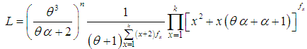 | (4.1) |
 | (4.2) |
 | (4.3) |
 | (4.4) |
 | (4.5) |
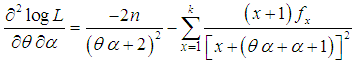 | (4.6) |
 | (4.7) |
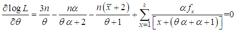
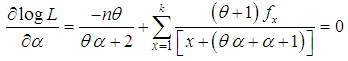
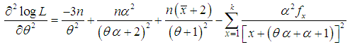
 of
of  of SBTPPLD (2.2), following equations can be solved
 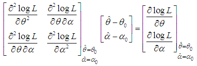 | (4.8) |
 and
and  being the initial values of
  and
and  are given by the method of moments. These equations are solved iteratively till sufficiently close estimates of
  and
and  are obtained.
4.2. Estimates from Moments
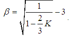
- The SBTPPLD has two parameters to be estimated and so the first two moments about origin are required to get the estimates of its parameters by the method of moments. From (3.2) and (3.3) we have
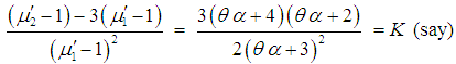 | (4.9) |
 , we get
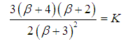 | (4.10) |
 | (4.11) |
 of
of  can be obtained.Again, substituting
  in (3.2) and replacing the population mean by the sample mean
  and
and  by
by  , moment estimate
  of
of  is obtained as
 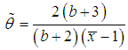 | (4.12) |
 of
of  is obtained as
 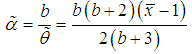 | (4.13) |
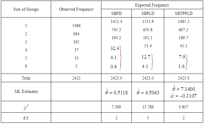
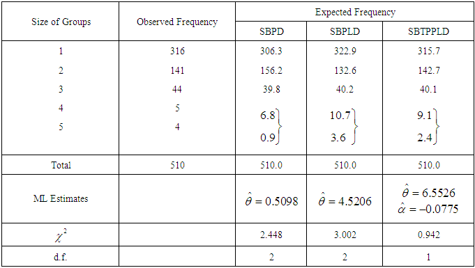
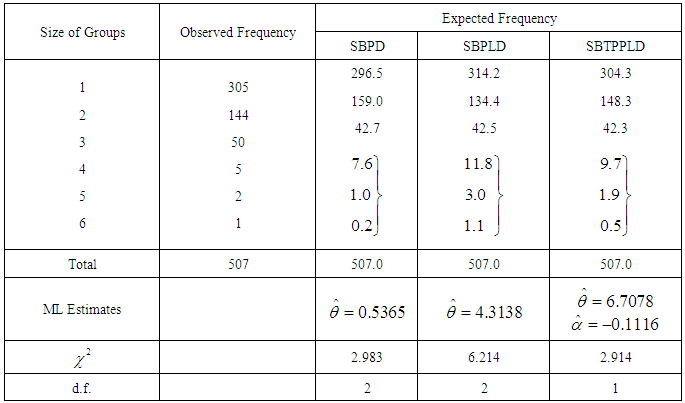
5. Goodness of Fit
- The SBTPPLD has been fitted to a number of data sets related to a number of observations of the size distribution of ‘freely –forming’ small groups in various public places reported by James (1953), Coleman and James (1961) and Simonoff (2003), and it was found that to almost all these data sets, the SBTPPLD provides closer fit than SBPD and SBPLD. Here, the goodness of fit of the SBTPPLD to three such data sets has been presented along with the goodness of fit given by SBPD and SBPLD.The expected frequencies according to the SBPD and SBPLD have also been given in these tables for ready comparison with those obtained by the SBTPPLD. The estimates of the parameters have been obtained by the method of maximum likelihood estimation. On the basis of the values of chi-square, it can be seen that the SBTPPLD gives much closer fit than those by the SBPD and SBPLD.The values of coefficient of variation (C.V), coefficient of skewness
 , coefficient of kurtosis
  and index of dispersion
  for estimated values of parameters for SBPD, SBPLD, and SBTPPLD and for original data for tables 1, 2 and 3 are presented in the following table 4.
|
|
|
|
 of SBPD, SBPLD, and SBTPPLD for estimated values of parameters and for original data
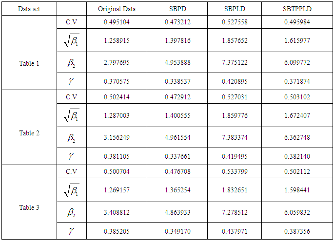
6. Conclusions
- In this paper, a size-biased two parameter Poisson-Lindley distribution (SBTPPLD), of which the size-biased Poisson-Lindley distribution (SBPLD) is a particular case, has been introduced to model count data which structurally excludes zero counts. The first four moments about origin, moments about mean, and expressions for coefficient of variation, skewness, kurtosis and index of dispersion have been obtained. The estimation of its parameters has been discussed using the method of maximum likelihood and the method of moments. The goodness of fit of the distribution has been presented to three data sets and it has been found that to all these data sets it provides much closer fit than both SBPD and SBPLD. The SBTPPLD has been found more general in nature and wider in scope than SBPD and SBPLD. Since SBTPPLD provides much closer fit to the observed data sets than those provided by the SBPD and SBPLD, SBTPPLD should be preferred over SBPD and SBPLD for modeling count data sets which structurally excludes zero counts.
ACKNOWLEDGEMENTS
- The authors are grateful to the Editor-In-Chief of the journal and the anonymous reviewer for constructive and helpful comments which lead to the improvement in the quality of the paper.