1. Introduction

If a variable is random, being independent and identically distributed (i.i.d.), it can be analyzed using standard statistical techniques such as the generalized linear models (GLMs). When the variable, however, is distributed in a manner that subjects it to systematic spatial variation, where observations at proximal locations are more similar than observations further apart, the independence assumptions of standard statistical methods fail. Parameters cannot easily be estimated via simple or straightforward statistical techniques such as the GLMs. Methods that allow for spatial dependency in the data are instead required for parameter estimation.

When the variable is also categorical, and ordered, modelling is further complicated, requiring complex inferential techniques to effectively handle the multiple categories, and also account for the ordering.

Premising the discourse on poverty this way is important, especially in light of the fact that welfare data are often

dominated by categorical observations collected (via living standards surveys) at several locations across space, and proximity of these observations imposes geographical structure on the data. This means that global parameters (obtained via independence assumptions of standard statistical methods) cannot adequately describe site-specific conditions of the variable.

Previous works to investigate poverty is abundant [1-5], but have largely ignored spatial dependence of observations and used methods that rely on independence assumptions, albeit with varying degrees of sophistication. This is problematic because when a regression model incorrectly assumes homoscedasticity in the errors of a spatial variable, outcome of the analysis can be biased [6].

The existing literatures [7-9] that have used spatial tools to study poverty have also largely ignored the multi-categorical and ordinal nature of the variable. Binary models for poverty analysis mask the effect of important intermediate information during the binary transformation of the variable [10], but also excludes the severest form of the variable; extreme poverty. This has the potential for incomplete and inaccurate description of poverty. The method for poverty analysis must be careful to explain why some population groups are non-poor, poor, or extremely poor.

So, what we do differently is to first discretize poverty into a multi-category ordered random variable using the severity levels as thresholds, and employ multivariate ordered analysis to describe the overall condition of a household as either being non-poor, poor, or extremely poor. Ordinal models solve the problem of loss of information during discretization by appealing to the concept of latent variables [11, 12], where a Gaussian random variable is assumed to be latent, and assigning values to the ordered categories according to a regression function.

Second, we assume that poverty, like all spatial phenomena, is not only a function of covariates, but also of unobservable large-scale interaction of geographical and agro-climatic forces.

Thus, we model poverty-severity risk as a spatially-varying ordinal phenomenon. Three models were proposed: The simple Ordinal Probit (OP) model [11], ordinal Spatial Generalized Linear Mixed Model (SGLMM) [12-14], and Clipped Gaussian Spatial Ordinal Probit (CG-SOP) model [15-17]. All the models were implemented in R version 3.1.3 [18], and ArcGIS [19].

To solve the inferential problems associated with spatial ordered models, we follow [20] to use the Bayesian decision paradigm, implemented via Markov Chain Monte Carlo (MCMC) sampling techniques.

Overall, our method can be considered a (category and site)-specific report that identifies all segments of the poor for easy targeting, thus avoiding the blanket approach that prefers the one-fits-it-all solution to the problem of poverty.

2. Measurement of Poverty

Poverty has many dimensions, but is generally measured in non-monetary or monetary terms [18]. We adopt the monetary approach to capture and report information in a form which facilitates comparison of our findings with similar international research.

Estimation of monetary poverty requires a choice between disposable income and total consumption expenditure as the indicator of wealth, the latter being the preferred choice in most developing countries [21], and in this study. Moreover, to measure monetary poverty, we need to set minimum standards of the poverty indicator to separate the various categories of the poor. These are called poverty lines [21]. The three categories of poverty lines adopted by [21] are based on family daily expenditure per adult equivalent. The thresholds are set at GHC 3.60 per day- non-poor, between GHC3.60 and GHC2.17–poor, and less than GHC2.17- extremely poor.

3. Data Sources and Covariates

The study used secondary data from the Ghana Living Standard Survey (GLSS). Included in the dataset of 16772 sampled households are details of households (household size, age, sex, and educational level of household head), socio-economic conditions of household (availability of social amenities), and neighbourhood information (ecological zone, rural/urban residence, and other environmental factors). The dataset of the GLSS collected in 2012 were not geo-coded. To perform spatial analysis, we geo-located each sampled household randomly (assuming a uniform distribution) at the district level in order to be consistent with existing spatial units.

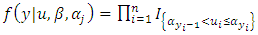
4. Ordinal Random Variables and Computations

4.1. The Ordinal Probit (OP) Model

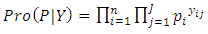
The traditional OP GLM [12] derives from the multinomial distribution, albeit with ranked categories. The density function for the multinomial distribution is:

(1)

where is the vector of responses, and constitutes the probability of observation being in category Here, the order of the outcomes is not important.

To derive the proportional odds cumulative OP GLM from (1), let the responses be arranged in order of magnitude, and be the corresponding thresholds associated with the ordering. Further let be a Gaussian random variable assumed to be latent, and assigning values to according to the regression function:

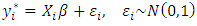(2)

where is design matrix, and is a unknown vector of regression coefficients, and is the vector of independently and identically distributed measurement errors: Though the values of cannot be directly observed, the rule that assigns to is that if exceeds a given threshold, then, an observation falls in the category. This culminates in cumulative multiple binary outcomes:

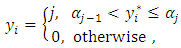(3)

where is the vector of response, and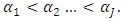

Clearly, in our application, refers to the Gaussian expenditure line, and is asymptotic of the ordinal variable when

Our objective is to predict the probability of a household falling in the category given the observed covariates This probability is determined by the values of the latent variable and is given by

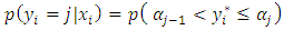(4)

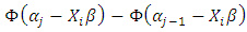
Since is Gaussian, and the outcome is a probit model, implying that the probability of falling in the category is:

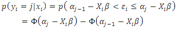(5)

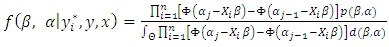
where is the cumulative distribution function for the normal Thus, the likelihood function for the parameters is

(6)

Several normalizations are needed to identify the ordered model parameters. For details see [12].

4.1.1. Bayesian Estimation via MCMC

Following the Bayesian criteria, we set priors for the parameters, and build the posterior as:

(7)

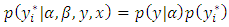
where is the data likelihood, is the prior density of model parameters, and is the integrated likelihood, with being the parameter space.

Posterior estimation is done by setting up the Gibbs sampler [14], which requires us to derive full conditionals for all parameters. We impose, following [12], non-informative priors on the regression coefficients. Then

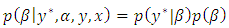(8)

(9)

(10)

where is the vector of observed ordinal outcomes, whiles is latent, is an indicator variable, leading to:

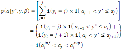(11)

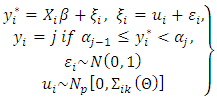
4.2. Spatial Measurement Framework

If, for example, ordinal observations are made at sites 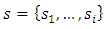under geo-statistical assumptions, then the data is defined as where and respectively are observations and response levels.

Let be the vector of associated covariates. Intuitively then,

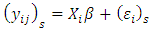(12)

spatial regression equations are written, where are -dimensional covariates, a vector of coefficients, and a spatially-dependent error. Let 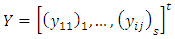, , and 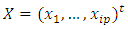, then equation (12) is written in matrix form as:

(13)

Spatial dependence is imposed by assuming that for where is a non-diagonal symmetric and positive definite matrix.

4.2.1. Spatial Generalized Linear Mixed Model (SGLMM)

The framework of the ordinal SGLMM is:

(14)

where is an design matrix, is a matrix of fixed effects coefficients, and spatially-dependent errors that capture all unobserved errors arising from the influence of common features for observations within certain proximal distances. The element of the spatial covariance matrix is parameterized by

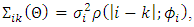(15)

where represents variability of the spatial process, and is a monotonic correlation function with a correlation decay parameter measuring the strength of spatial dependence over the Euclidean distance between locations and [22].

By maintaining the ordinal probit form, and assuming, following [22], that the spatial error term also represents random measurement error in unexplained explanatory variables (the nugget), then

(16)

Thus, the likelihood function is

(17)

where is an indicator function equalling 1 when and 0 otherwise.

4.2.1.1. Bayesian Estimation via MCMC

Using the Bayesian approach [17], the posterior likelihood is:

(18)

where is the data vector, is latent regression function assigning values to observable ordered data, is distribution of the latent errors incorporated via data augmentation, and are prior densities for the model parameters.

The use of MCMC sampling, especially Gibbs techniques [20], requires us to derive full conditionals for all parameters. We assume following [22] non-informative priors for the regression coefficients and inverse gamma for the spatial parameters. Thus, the full conditionals of all parameters have the following functional forms:

(19)

(20)

(21)

(22)

(23)

(24)

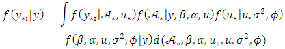
4.2.2. The CG-SOP Model

To create a workable geo-statistical framework, we define an ordinal random field by assuming that the spatially-dependent errors are latent, but together with some covariates, are assigning values to according to the multivariate regression function:

(25)

where variables and parameters are as previously defined. The element of is parameterized by 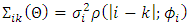, where parameters are as previously defined.

The link between and is seen by assuming that for a vector of thresholds the ordinal random field, is obtained by quantizing at levels thus, culminating in multiple binary outcomes:

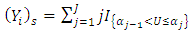(26)

where

Our objective is to model the probability of an observation at site falling at the category. This probability is determined by

(27)

Now, is n-dimensional, and determined by the density of Therefore, the likelihood of the data is the integral of an n-dimensional multivariate normal distribution taking values in the interval

(28)

4.2.2.1. Bayesian Estimation via MCMC

Following the Bayesian methodology [20], the full joint posterior distribution for all unknown parameters is completely defined by the posterior likelihood:

(29)

where is an indicator variable, and being the joint prior density, specifies uncertainty on the respective estimated parameters. We complete the specification by imposing non-information priors on the regression parameters and inverse gamma on the spatial parameters [16, 17].

The full conditional posterior distributions of each parameter [20] have the following functional forms:

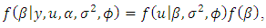(30)

(31)

(32)

(33)

(34)

At this point, all parameters of interest are sampled sequentially via MCMC simulation until the desired number of draws is achieved.

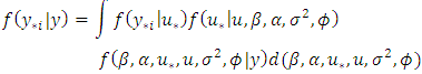
4.3. Posterior Predictions and Mapping

A key goal of this study is to produce a smooth map of household poverty-severity risk in Ghana by predicting the outcome at new locations. We achieve this via kriging [23-25].

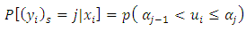
Define to be the map of predictive ordered responses corresponding to poverty-severity risk at unsampled locations 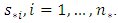The predictions are derived from the conditional probabilities that a new location falls in category given the observed data. In ordered modelling, these conditional probabilities cannot be obtained via direct MCMC simulations; they are obtained by calculating 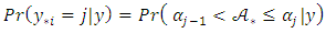using MCMC integration and data augmentation, where is a latent variable at new locations, being equal to in both OP GLM and SGLMM, and for the CG-SOP model.

Following the Bayesian approach, the predictive posterior distributions is augmented by to give:

(35)

in the case of the aspatial OP GLM,

(36)

for the SGLMM, and for the CG-SOP case, we have

(37)

4.4. Model Evaluation and Validation Measures

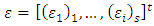
The posterior predictive densities are the distribution of possible future observations arising from the current model. We determine a checking function for both predicted data and actual observations to assess predictive model fit. In line with this, we proceed by first randomly splitting the dataset into two equal parts: one part (8375) as training set and the other (8375) as a validation set [26].

In standard ML analyses, a repertoire of fit measures includes and likelihood-ratio statistic. In Bayesian analyses, predictive model selection is checked within the framework of Bayesian decision theory [26, 27, 20], where prediction accuracy is based on the Bayesian expected loss (BEL). The loss function represented here by the additive loss function estimates the loss incurred in predicting by at location; assigning zero loss to correct predictions. For the multi-categorical application, the additive loss function in respect of new locations is expressed as:

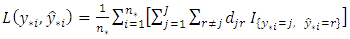(38)

where penalizes the loss incurred for mis-predicting category when the true category is If is set to 1, equation (38) translates to the well-known mis-prediction rate (MPR) (defined as the proportion of predictions that are incorrect), and optimal Bayes’ prediction is attained by choosing the value for that minimizes (38), leading to the expected value of the loss function:

(39)

Equation (39) corresponds to the value of that reports the highest estimated probability.

In assessing the models, it is important to note the difference between the estimated BEL (using the training data) and validation BEL (using the validation data) for each model. A comparatively large difference shows a model is making incorrect predictions [26, 20].

For the ordered data, it is also possible for the model to suffer greater loss for predictions that are farther from the truth. Thus, we assign loss coefficients and get the absolute mis-prediction rate (AMPR) defined as:

(40)

where is the true value and is the prediction. In principle, the AMPR accounts for the size of the mis-prediction.

We apply all the fit measures (MPR, AMPR, and BEL) to determine the models’ ability to correctly forecast future values.

5. Results

Before proceeding to perform spatial analysis, we need to confirm that the data exhibits significant spatial correlation. In this regard, the simple OP GLM was fitted to the data. Although spatial correlation in the raw data is of interest, we were primarily interested in whether there was correlation in model residuals once any correlation explained by the explanatory variables has been accounted for by the simple OP GLM. Figure 1 shows the classical semi-variogram estimator by [24], which is based on the residuals obtained after fitting the GLM.

It is clear from Figure 1 that there is a spatial trend beyond what was described by the mean structure alone. The semi-variogram shows an increasing trend from the origin, indicating lag-dependent variation. Therefore we expect high variability in the covariance parameters.

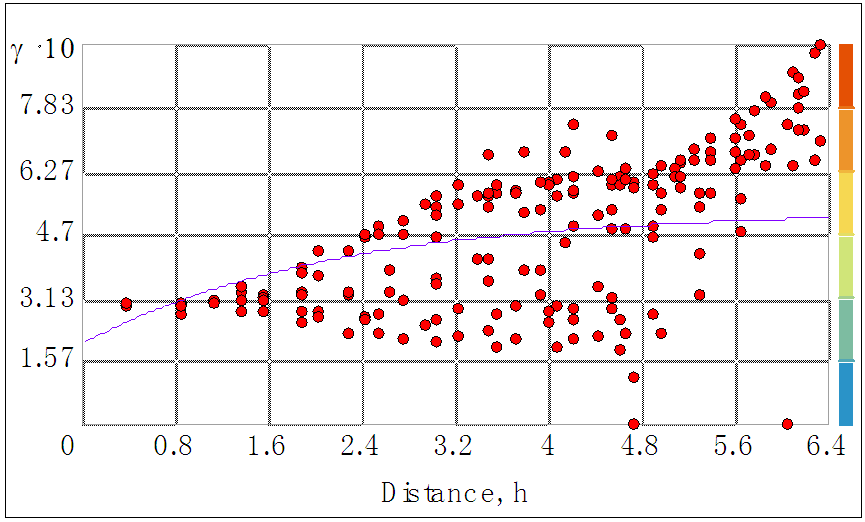Figure 1. Classical Semi-Variogram

Table 1 presents estimation results for posterior means and 95% Bayesian credible intervals (BCIs) to compare performance of the three different OP models. The value 0 in the range of the BCI means that the parameter is not significant.

Table 1. Comparison of Posterior Estimates using the Different OP Model Specifications

Estimates of the beta coefficients differ significantly among the three models. The posterior means for the spatial models (SGLMM and CG-SOP) appear smaller than those from the aspatial OP GLM. Perhaps, this confirms that some of the spatial dependence is explained by the correlation functions whereas these functions are absent in the aspatial model.

Differences were also observed between the competing spatial models. While the SGLMM estimates to be 0.035, the CG-SOP model estimate of is 0.041. These disparities are largely due to the differential parameterizations used for each model.

We use the estimate to determine the effective range of spatial correlation, commonly defined as the distance beyond which the correlation reduces to less than 5% of variance. For the exponential correlation function, the effective range is for the SGLMM, and for the CG-SOP model [20]. Thus, the estimated effective range for the response surface of the SGLMM is 66 kilometers, suggesting lower spatial variation compared to the CG-SOP model with an effective range of 73 kilometers. Though both models appear to exhibit large ranges relative to the maximum inter-site distance of 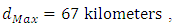the CG-SOP model does better at larger lags (see Figures 2 and 3).

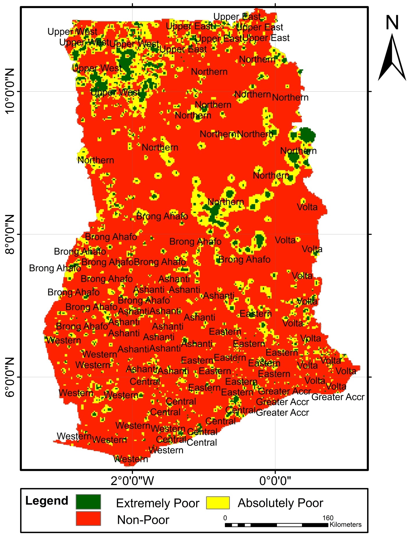Figure 2. Poverty-Severity Map of Ghana Using the SGLMM

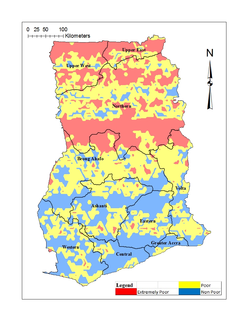Figure 3. Poverty-Severity Map of Ghana using the CG-SOP Model

Regarding our application, the estimation results (Table 1) show that, for the spatial models, all the risk factors are well within the 2.5% and 97.5% percentiles; being significantly different from 0. This shows clearly that these models were very successful at capturing key features of the observed data, thus, providing correct conclusions about the association between poverty-severity and the predictor variables.

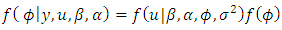
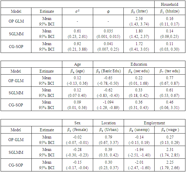
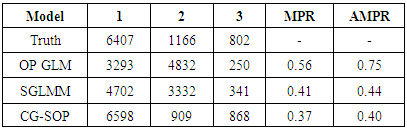
The estimate in all three models shows a positive link between household size and poverty severity, showing that poverty severity levels tend to increase from non-poor to extremely poor for sites with higher household sizes. Age was found not statistically significant in the OP GLM. Higher education was found to reduce the risk of extreme poverty in all three models. Extreme poverty-risk was also related to the residency of household head, with urbanites being at lower risks of extreme poverty. The impact employment has on poverty-risk in this study is typical; showing lowest risk for wage employed householders in the SGLMM and CG-SOP models. Its effect in the non-spatial OP GLM was however mixed. Unemployed was found not to be statistically significant in this model.

Table 2 summarizes and compares results for predictive abilities whiles Table 3 does same for Bayesian expected loss (BEL) for each specification.

Clearly, results of Table 2 identified the CG-SOP as the preferred model for prediction. Its predicted values come closest to the truth compared to the aspatial cumulative OP GLM and the SGLMM. Closely following the CG-SOP in predictive performance is the SGLMM. Thus, incorporating spatial dependence in the modelling framework improves estimation and prediction as evidenced by the performance of the two spatial models.

Table 2. Validation Test on the Three OP Models using Measures of MPR and AMPR

For ordered models, values of AMPR provide information about how far the mis-predictions are from the true category. The OP-GLM is the worst performing in this regard, followed by the SGLMM (Table 2). The proportion of mis-predictions exceeding one category is 0.75 for the OP-GLM, reducing to 0.40 for the SG-SOP model.

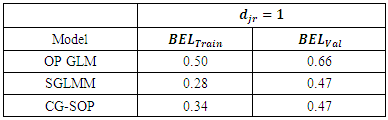
A further comparison of predictive performance of the models was made using Bayesian expected loss (BEL). Calculations were based on training and validation data. A significantly large difference between and indicates a model is mis-predicting the outcomes [26]. Table 3 presents results of the analysis, showing the OP-GLM and SGLMM as culprits in this regard. The CG-SOP has the smallest difference between and

Table 3. Validation Test on the Three OP Models using Measures of BEL

Overall, all the fit statistics suggest that the CG-SOP model more accurately estimates the parameters, with a better fit to the observed data, and should be preferred.

Predictions of poverty-severity risk, using the spatial models (SGLMM and CG-SOP), were made at unobserved locations across all ten regions of Ghana. Each thresholding level of the models was represented by a specific colour, thus thresholding at three levels produced a three-colour poverty severity map shown in Figures 2 and 3 respectively for the SGLMM and CG-SOP.

The predicted map exposes relatively large regional differences. The map shows higher concentration of extreme poverty in the northern part of the country, extending to the transitional belt of the savannah ecological zone, along the border with Brong Ahafo Region. Large fluctuations are however observed within the Ashanti and Greater Accra regions and environs.

6. Discussion

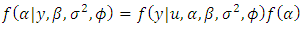
Geo-statistical OP models that ordered the population into three distinct categories (non-poor, poor, and extremely poor) were employed. The models were built to forecast the risk of regional household poverty-severity in Ghana.

Inference compared MCMC simulations from the aspatial OP GLM and ordinal SGLMM with the CG-SOP model. The large difference in predictive ability between the aspatial and the spatial models confirms the limitation of the simple OP GLM, and by extension, all aspatial models when dealing with spatial correlation in geo-referenced data.

Bayesian inference via MCMC produced estimates of spatial parameters and subsequently, posterior predictive probabilities at unobserved sites. It is difficult to see how traditional aspatial methods such as the ordinary least squares (OLS) would estimate spatial parameters. The OP GLM for instance, though easy to formulate and estimate, does not sufficiently exploit sample information, thus producing biased results. Although the 95% confidence intervals (CIs) for the betas of the OP GLM (Table 1) were consistently narrower, this was hard to believe. Of course, as sample size increases, the CIs correspondingly decrease. However, if the increase in sample size results from the inclusion of more heterogeneous observations, narrowing of the CIs is anomalous.

The CG-SOP model results, summarized by the 95% credible intervals, and associated spatial parameters and show a relatively stronger spatial dependence. Results of the ordinal SGLMM are similarly distributed. However, the SGLMM overestimates suggesting a lower spatial variation than the CG-SOP model, especially at large lags (Figures 2 and 3). The results thus suggest that the CG-SOP is the preferred model for estimation and prediction.

Regarding our application, higher levels of extreme poverty is predicted in most of the northern half of the country, extending to the borders with Togo, Cote d'Ivoire, and Burkina Faso. This region lies in the dry savannah ecological zone with short seasonal rainfalls, rendering agricultural lands unproductive for the predominantly farming populations in the area.

Low poverty is predicted in much of the forested south and coastal parts of the country. The Greater Accra region is predicted with the lowest risk of extreme poverty, as expected. The seaports and heavy industrial plants (along with the recently discovered crude oil) are found predominantly across the middle and coastal belts of the country, where both the rich agricultural lands and tropical rain forest coincide. Heavy mining of gold, diamond and other mineral resources over the last half-century have all contributed significantly to the low levels of poverty predicted at various locations in the south of the country.

However, pockets of poverty observed at different scales in the southernmost parts of the country reflect urban and peri-urban deprivations. These could be due to disturbances linked to short range environmental factors, reiterating the fact that even over much smaller distances, local disturbances can have a distinct effect on the distribution of the poor.

The spatial disparities of poverty-severity revealed by this study conform to expert opinion that in a geographic environment, there can be a dominant non-stochastic relationship between economic wellbeing and the spatial dynamics of a country [28, 29].

Application of the modelling techniques to the socio-econometric problem considered here is novel, and demonstrates our contribution to the wider scope of spatial-statistical methods. We model multi-categorical socio-econometric data in a spatial measurement framework that recognizes the ordinal nature of the variable. In our application, we depart from the auto regressive (AR) approach by directly embedding the ordinal variable within the distributional framework of a latent spatial GRF, and this marks a significant innovation.

7. Conclusions and Recommendations

An integral objective of this study was to improve prediction, especially when the data is collected over large geographical areas. The results suggest that the CG-SOP model is well suited to this objective.

The study has identified positive correlation with respect to the distribution of poverty. Individuals in specific locations tend to uniformly experience specific categories of poverty regardless of their personal circumstances, thus, providing an empirical spatial character of poverty in Ghana. We see a pictorial evidence of this in the predictive maps (Figures 1 and 2).

Poverty eradication efforts should be directed towards areas with high posterior ranks. For example, extreme poverty incidence in the Upper West and some areas at the border between the Northern and Brong Ahafo regions, extending eastwards, may be of concern. Conversely, stakeholders may wish to preserve areas with low incidence of extreme poverty.

8. Future Work

While we are satisfied with the CG-SOP model per our stated objectives, it needs to be noted that our model did not account for non-stationarity in the underlying spatial process. We assumed a stationary spatial process, meaning that spatial correlation between locations of the same distance remains the same throughout the region [30]. Non-stationarity allows both the data and covariates to vary spatially. Addressing non-stationarity further improves both model fit and prediction.