Rama Shanker1, Kamlesh Kumar Shukla1, Ravi Shanker2, Tekie Asehun Leonida3
1Department of Statistics, Eritrea Institute of Technology, Asmara, Eritrea
2Department of Mathematics, G.L.A. College, N.P University, Daltonganj, Jharkhand, India
3Department of Applied Mathematics, University of Twente, Enschede, The Netherlands
Correspondence to: Rama Shanker, Department of Statistics, Eritrea Institute of Technology, Asmara, Eritrea.
| Email: |  |
Copyright © 2017 Scientific & Academic Publishing. All Rights Reserved.
This work is licensed under the Creative Commons Attribution International License (CC BY).
http://creativecommons.org/licenses/by/4.0/

Abstract
A three-parameter Lindley distribution, which includes some two-parameter Lindley distributions introduced by Shanker and Mishra (2013 a, 2013 b), Shanker et al (2013), Shanker and Amanuel (2013), two-parameter gamma distribution, and one parameter exponential and Lindley distributions as special cases, has been proposed for modeling lifetime data. Its statistical properties including its shape, moments, skewness, kurtosis, hazard rate function, mean residual life function, stochastic ordering, mean deviations, order statistics, Renyi entropy measure, Bonferroni and Lorenz curves, stress-strength reliability have been discussed. For estimating its parameters, maximum likelihood estimation has been discussed. Finally, a numerical example has been presented to test the goodness of fit of the proposed distribution and the fit has been compared with the three-parameter generalized Lindley distribution.
Keywords:
Lindley distribution, Quasi Lindley distribution, Two-parameter Lindley distribution, Generalized Lindley distribution, Mathematical and Statistical properties, Moments, Maximum Likelihood estimation, Goodness of fit
Cite this paper: Rama Shanker, Kamlesh Kumar Shukla, Ravi Shanker, Tekie Asehun Leonida, A Three-Parameter Lindley Distribution, American Journal of Mathematics and Statistics, Vol. 7 No. 1, 2017, pp. 15-26. doi: 10.5923/j.ajms.20170701.03.
1. Introduction
The modeling and analyzing lifetime data are crucial in many applied sciences including medicine, engineering, insurance and finance, amongst others. During a short span of time a number of one parameter, two-parameter and three-parameter lifetime distributions have been introduced in statistical literature for modeling lifetime data from biomedical science and engineering. But each of these lifetime distributions has advantages and disadvantages over one another due to the number of parameters involved, shape, hazard rate function and mean residual life function, among others. Lindley (1958) distribution, introduced in the context of Bayesian analysis as a counter example of fiducial statistics, is defined by its probability density function (p.d.f) and cumulative distribution function (c.d.f) 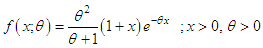 | (1.1) |
 | (1.2) |
A detailed study about its important mathematical and statistical properties, estimation of parameter and application showing the superiority of Lindley distribution over exponential distribution for the waiting times before service of the bank customers has been done by Ghitany et al (2008). Shanker et al (2015) have comparative study on modeling of lifetime data using one parameter Lindley (1958) distribution and exponential distribution and concluded that there are many lifetime data where exponential distribution gives better fit than Lindley distribution. Sankaran (1970) obtained a Poisson mixture of Lindley distribution and named it discrete Poisson-Lindley distribution (PLD) and discussed its various properties, estimation of parameter and goodness of fit. Shanker and Hagos (2015) have introduced a simple method for estimating parameter of PLD and discussed its applications for modeling count data from biological sciences. The probability density function (p.d.f.) and cumulative distribution function (c.d.f) of quasi Lindley distribution (QLD) of Shanker and Mishra (2013a) are given by  | (1.3) |
 | (1.4) |
At  , both (1.3) and (1.4) reduce to the corresponding expressions (1.1) and (1.2) of Lindley distribution. Shanker and Mishra (2016) have obtained a Poisson mixture of a quasi Lindley distribution and named it a ‘quasi Poisson-Lindley distribution (QPLD)’ and discussed its various statistical and mathematical properties, estimation of parameters, and applications. Shanker et al (2016 a) have discussed many interesting properties of QLD and its applications for modeling various lifetime data and observed that it gives better fit in most of the data sets.The probability density function (p.d.f.) and cumulative distribution function (c.d.f) of two-parameter Lindley distribution (TPLD) of Shanker and Mishra (2013b) are given by
 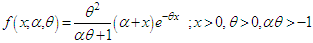 | (1.5) |
 | (1.6) |
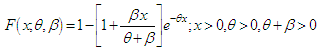
At  , both (1.5) and (1.6) reduce to the corresponding expressions (1.1) and (1.2) of Lindley distribution. Shanker and Mishra (2014) have obtained a Poisson mixture of a two- Lindley distribution and named it a two-parameter Poisson-Lindley distribution and discussed its various statistical and mathematical properties, estimation of parameters, and applications. Shanker et al (2016 b) have discussed many interesting properties of TPLD and its applications for modeling various lifetime data and observed that it gives better fit in most of the data sets.The probability density function (p.d.f.) and cumulative distribution function (c.d.f) of another two-parameter Lindley distribution, introduced by Shanker et al (2013) are given by
 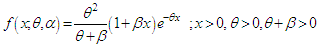 | (1.7) |
 | (1.8) |
At  , both (1.7) and (1.8) reduce to the corresponding expressions (1.1) and (1.2) of Lindley distribution. Shanker et al (2012) obtained a Poisson mixture of two-parameter Lindley distribution, named it a ‘discrete two-parameter Poisson-Lindley distribution’ and studied its various properties, estimation of parameters and applications.The probability density function (p.d.f.) and cumulative distribution function (c.d.f) of a new quasi Lindley distribution (NQLD), introduced by Shanker and Amanuel (2013) are given by
 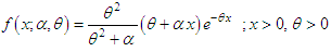 | (1.9) |
 | (1.10) |
Where  or
or  At
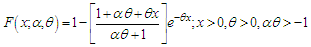
At  , both (1.9) and (1.10) reduce to the corresponding expressions (1.1) and (1.2) of Lindley distribution. Shanker and Tekie (2014) obtained a new quasi Poisson-Lindley distribution by taking a Poisson mixture of NQLD, discussed its various statistical and mathematical properties, estimation of parameters and applications for count data.The probability density function of three-parameter generalized Lindley distribution (TPGLD) introduced by Zakerzadeh and Dolati (2009) having parameters
  is given by
 | (1.11) |
Clearly the gamma distribution, the Lindley (1958) distribution and the exponential distribution are particular cases of (2.1) for  respectively. The discussion about its properties, estimation of parameters and applications are available in Zakerzadeh and Dolati (2009). The corresponding distribution function of the TPGLD can be obtained as
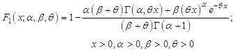 | (1.12) |
where  is the upper incomplete gamma function defined as
 Recently Shanker (2016) has detailed study about TPGLD and obtained expressions for coefficient of variation, skewness, kurtosis, index of dispersion, hazard rate function and the mean residual life function. Shanker (2016) has detailed comparative study of TPGLD and three-parameter generalized gamma distribution (TPGGD) and observed that in most of the data sets from medical science and engineering TPGGD gives better fit than TPGLD.There are many situations where these distributions are not suitable for modeling lifetime data from theoretical or applied point of view. Therefore, an attempt has been made in this paper to obtain a new distribution which is flexible than these lifetime distributions for modeling lifetime data in reliability and in terms of its hazard rate shapes. Various interesting mathematical and statistical properties of the proposed distribution have been discussed. The estimation of the parameters of the proposed distribution has been discussed using maximum likelihood estimates and the goodness of fit of the distribution has been discussed with a real lifetime data. Finally the goodness of fit of the proposed distribution has been compared with three-parameter generalized Lindley distribution, introduced by Zakerzadeh and Dolati (2009).
2. A Three-Parameter Lindley Distribution
The probability density function (p.d.f.) of a three- parameter Lindley distribution (ATPLD) can be introduced as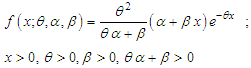 | (2.1) |
It can be easily verified that the two-parameter quasi Lindley distribution of Shanker and Mishra (2013 a), two-parameter Lindley distribution of Shanker and Mishra (2013 b), two-parameter Lindley distribution of Shanker et al (2013), a new two-parameter quasi Lindley distribution of Shanker and Amanuel (2013), Lindley distribution introduced by Lindley (1958), Gamma  distribution and exponential distribution are particular cases of a three-parameter Lindley distribution (ATPLD) for
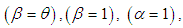
 and
and  respectively.This distribution can be easily expressed as a mixture of exponential
  and gamma
  distributions with mixing proportion
  We have
 where
where 
 and
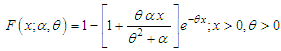
and The corresponding cumulative distribution function (c.d.f.) of (2.1) is given by
 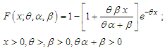 | (2.2) |
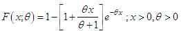
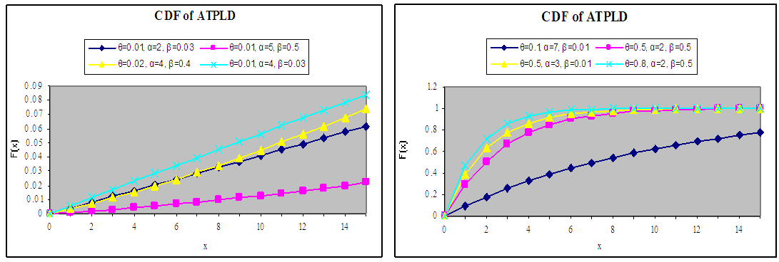
The graph of the p.d.f. and the c.d.f. of ATPLD for different values of  are shown in figures 1 and 2.
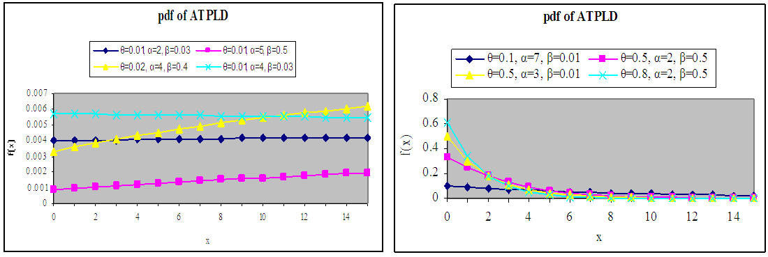 | Figure 1. Graph of the pdf of ATPLD for different values of parameters  |
 | Figure 2. Graph of the cdf of ATPLD for different values of parameters  |
3. Statistical Constants
The  moment about origin of ATPLD (2.1) can be obtained as
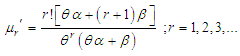 The first four moments about origin of ATPLD are as follows
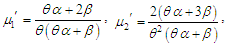
 Thus the moments about mean of ATPLD are obtained as
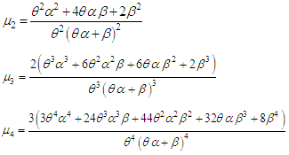 The coefficient of variation
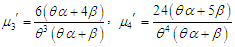
 coefficient of skewness
  coefficient of kurtosis
  and index of dispersion
  of ATPLD are thus obtained as
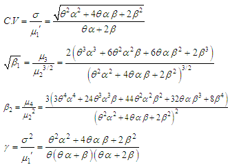
4. Hazard Rate Function and Mean Residual Life Function
Let  and
and  be the p.d.f. and c.d.f of a continuous random variable. The hazard rate function (also known as the failure rate function) and the mean residual life function of
  are respectively defined as
 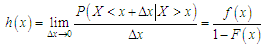 | (4.1) |
and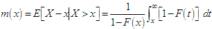 | (4.2) |
The corresponding hazard rate function,  and the mean residual life function,
  of ATPLD are obtained as
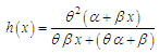 | (4.3) |
and 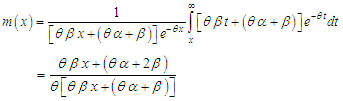 | (4.4) |
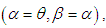
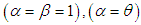
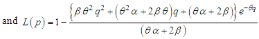
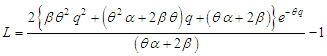
It can be easily verified that 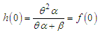 and
and 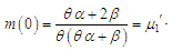 It is also obvious from the graphs of
  and
and  that
that  is an increasing and decreasing functions of
  and
and  whereas
  is a decreasing function of
  and
and  The graph of the hazard rate function and mean residual life function of ATPLD are shown in figures 3 and 4.
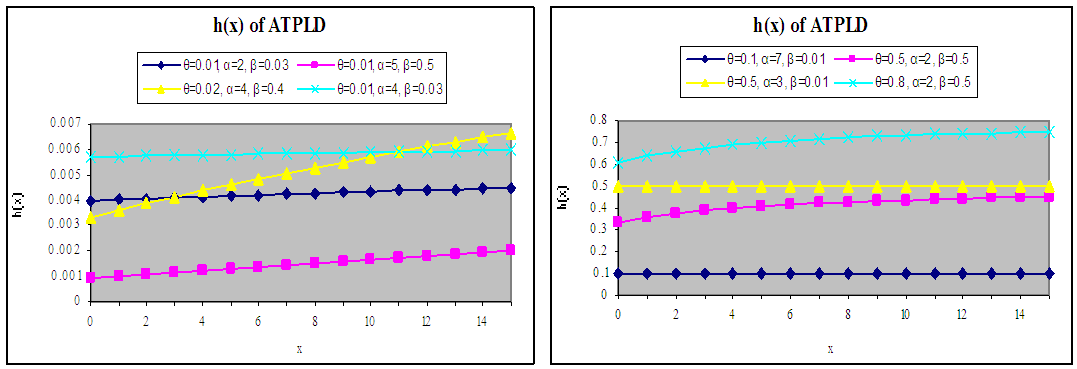 | Figure 3. Graph of hazard rate function of ATPLD for different values of parameters  |
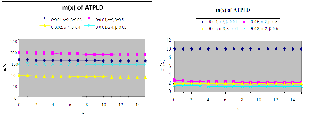 | Figure 4. Graph of mean residual life function of ATPLD for different values of parameters  |
5. Stochastic Orderings
Stochastic ordering of positive continuous random variables is an important tool for judging their comparative behavior. A random variable  is said to be smaller than a random variable
  in the (i) stochastic order
  if
if  for all
  (ii) hazard rate order
  if
if 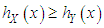 for all
  (iii) mean residual life order
  if
if  for all
  (iv) likelihood ratio order
  if
if  decreases in
  The following results due to Shaked and Shanthikumar (1994) are well known for establishing stochastic ordering of distributions
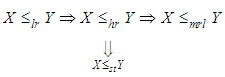 | (5.1) |
The ATPLD is ordered with respect to the strongest ‘likelihood ratio’ ordering as shown in the following theorem:Theorem: Let  and
and 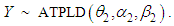 Now under conditions (i)
 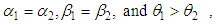 (ii)
(ii) 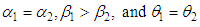 and (iii)
 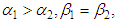 and
and  and hence
  and
and  Proof: We have
  Now
Now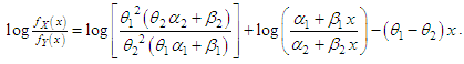 This gives
 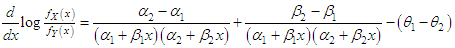 It can be easily verified that under conditions (1), (ii), and (iii),
  This means that
  and hence
  and
and 
6. Mean Deviations
The amount of scatter in a population is measured to some extent by the totality of deviations usually from mean and median. These are known as the mean deviation about the mean and the mean deviation about the median defined by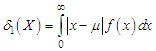 and
and 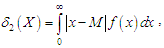 respectively, where
  and
and 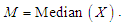 The measures
  and
and  can be calculated using the relationships
 | (6.1) |
and  | (6.2) |
Using p.d.f. (2.1) and expression for the mean of ATPLD, we get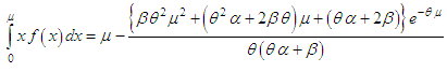 | (6.3) |
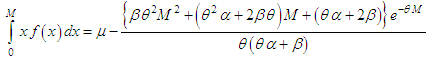 | (6.4) |
Using expressions from (6.1), (6.2), (6.3), and (6.4), the mean deviation about mean,  and the mean deviation about median,
  of ATPLD are obtained as
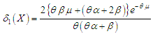 | (6.5) |
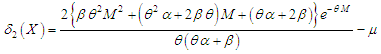 | (6.6) |
7. Bonferroni and Lorenz Curves
The Bonferroni and Lorenz curves (Bonferroni, 1930) and Bonferroni and Gini indices have applications not only in economics to study income and poverty, but also in other fields like reliability, demography, insurance and medicine. The Bonferroni and Lorenz curves are defined as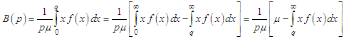 | (7.1) |
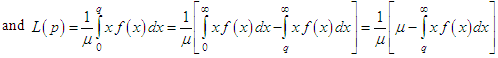 | (7.2) |
respectively or equivalently  | (7.3) |
 | (7.4) |
respectively, where  and
and  The Bonferroni and Gini indices are thus defined as
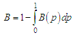 | (7.5) |
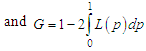 | (7.6) |
respectively.Using p.d.f. (2.1), we get 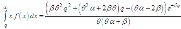 | (7.7) |
Now using equation (7.7) in (7.1) and (7.2), we get 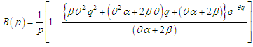 | (7.8) |
 | (7.9) |
Now using equations (7.8) and (7.9) in (7.5) and (7.6), the Bonferroni and Gini indices of ATPLD are obtained as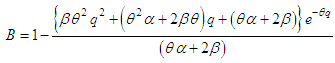 | (7.10) |
 | (7.11) |
8. Order Statistics and Renyi Entropy Measure
8.1. Order Statistics
Let  be a random sample of size
  from ATPLD (2.1). Let
  denote the corresponding order statistics. The p.d.f. and the c.d.f. of the
  order statistic, say
  are given by
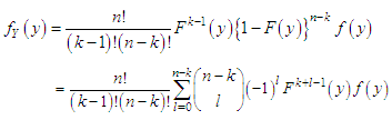 and
and 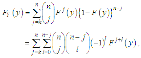 respectively, for
 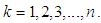 Thus, the p.d.f. and the c.d.f of
  order statistics of ATPLD are obtained as
 and
and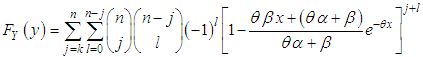
8.2. Renyi Entropy Measure
An entropy of a random variable  is a measure of variation of uncertainty. A popular entropy measure is Renyi entropy (1961). If
  is a continuous random variable having probability density function
  then Renyi entropy is defined as
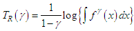 where
where 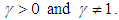 Thus, the Renyi entropy for ATPLD (2.1) can be obtained as
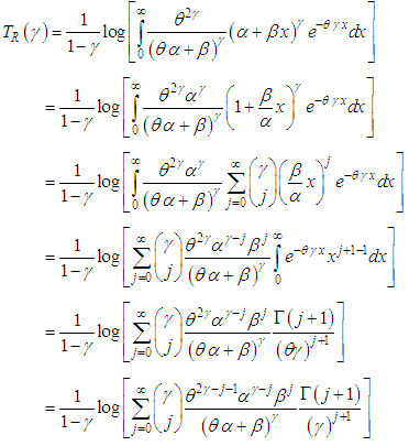
9. Stress-Strength Reliability
The stress- strength reliability describes the life of a component which has random strengththat is subjected to a random stress  When the stress applied to it exceeds the strength, the component fails instantly and the component will function satisfactorily till
  Therefore,
  is a measure of component reliability and in statistical literature it is known as stress-strength parameter. It has wide applications in almost all areas of knowledge especially in engineering such as structures, deterioration of rocket motors, static fatigue of ceramic components, aging of concrete pressure vessels etc.Let
  and
and  be independent strength and stress random variables having ATPLD (2.1) with parameter
  and
and  respectively. Then the stress-strength reliability
  of ATPLD can be obtained as
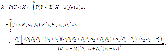
10. Maximum Likelihood Estimate (MLE)
Let  be a random sample of size
  from ATPLD (2.1). The likelihood function,
  of (2.1) is given by
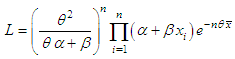 The natural log likelihood function is thus obtained as
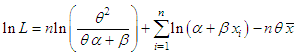 The maximum likelihood estimates (MLE)
  and
and  and
and  are then the solutions of the following non-linear equations
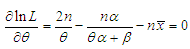 | (10.1.1) |
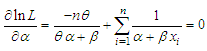 | (10.1.2) |
 | (10.1.3) |
where  is the sample mean. The equation (10.1.1) gives
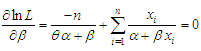
  which is the mean of ATPLD (2.1). These three natural log likelihood equations do not seem to be solved directly. However, the Fisher’s scoring method can be applied to solve these equations. We have
 The following equations can be solved for MLEs
  and
and  of
of  and
and  of ATPLD
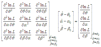 where
where  and
and  are the initial values of
  and
and  respectively. These equations are solved iteratively till sufficiently close values of
  and
and  are obtained.
11. Goodness of Fit
A three-parameter Lindley distribution (ATPLD) has been fitted to a number of lifetime data to test its goodness of fit. In this section, we present the goodness of fit of ATPLD for a real lifetime data and its fit has been compared with the three-parameter generalized Lindley distribution (TPGLD), introduced by Zakerzadeh and Dolati (2009). The following lifetime data has been considered for testing the goodness of fit of ATPLD and TPGLD.Data Set: This data represents the survival times (in days) of 72 guinea pigs infected with virulent tubercle bacilli, observed and reported by Bjerkedal (1960)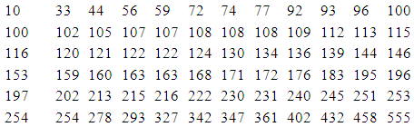 In order to compare ATPLD and TPGLD, values of
  and K-S Statistics (Kolmogorov-Smirnov Statistics) for real life time data has been computed. The formulae for computing K-S Statistics is as follows:
 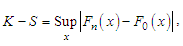 where
where  = the number of parameters,
  = the sample size and
  is the empirical distribution function. The best distribution is the distribution which corresponds to lower value of
  and K-S statistics and higher p-value.
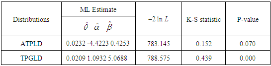
Table 1. MLE’s, - 2ln L, AIC, AICC, BIC, and K-S Statistics of the fitted distributions of data
 |
| |
|
It can be easily seen from above table that ATPLD gives better fit than the TPGLD, introduced by Zakerzadeh and Dolati (2009).
12. Concluding Remarks
A three-parameter Lindley distribution (ATPLD) which includes two-parameter Lindley distributions introduced by Shanker and Mishra (2013 a, 2013 b) , Shanker et al (2013), Shanker and Amanuel (2013), two-parameter gamma distribution, and one parameter exponential and Lindley distributions, has been introduced for modeling lifetime data. Its mathematical and statistical properties including its shape, moments, skewness, kurtosis, hazard rate function, mean residual life function, stochastic ordering, mean deviations, order statistics, Renyi entropy measure, Bonferroni and Lorenz curves, stress-strength reliability have been discussed. For estimating its parameters, maximum likelihood estimation has been discussed. The goodness of fit of ATPLD has been found better than the goodness of fit given by TPGLD, and hence ATPLD can be considered an important lifetime distribution for modeling lifetime data over TPGLD.
ACKNOWLEDGEMENTS
The authors are grateful to the editor-in-chief of the journal and the anonymous reviewer for constructive comments which lead to the improvement in the quality of the paper.
References
| [1] | Bjerkedal, T. (1960): Acquisition of resistance in guinea pigs infected with different doses of virulent tubercle bacilli, American Journal of Epidemiology, 72 (1), 130 -148. |
| [2] | Bonferroni, C.E. (1930): Elementi di Statistca generale, Seeber, Firenze. |
| [3] | Ghitany, M.E., Atieh, B. and Nadarajah, S. (2008): Lindley distribution and its Application, Mathematics Computing and Simulation, 78, 493 – 506. |
| [4] | Lindley, D.V. (1958): Fiducial distributions and Bayes’ theorem, Journal of the Royal Statistical Society, Series B, 20, 102- 107. |
| [5] | Sankaran, M. (1970): The discrete Poisson-Lindley distribution, Biometrics, 26, 145 - 149. |
| [6] | Shaked, M. and Shanthikumar, J.G. (1994): Stochastic Orders and Their Applications, Academic Press, New York. |
| [7] | Shanker, R (2016): On generalized Lindley distribution and its applications to model lifetime data from biomedical science and engineering, to appear in, “Insights in Biomedicine”. |
| [8] | Shanker, R. and Mishra, A. (2013 a): A quasi Lindley distribution, African Journal of Mathematics and Computer Science Research, 6(4), 64 – 71. |
| [9] | Shanker, R. and Mishra, A. (2016): A quasi Poisson- Lindley distribution, to appear in Journal of Indian Statistical Association. |
| [10] | Shanker, R. and Mishra, A. (2013 b): A two-parameter Lindley distribution, Statistics in Transition-new series, 14 (1), 45- 56. |
| [11] | Shanker, R. and Mishra, A. (2014): A two-parameter Poisson-Lindley distribution, International Journal of Statistics and Systems, 9(1), 79 – 85. |
| [12] | Shanker, R., Sharma, S. and Shanker, R. (2013): A two-parameter Lindley distribution for modeling waiting and survival times data, Applied Mathematics, 4, 363 – 368. |
| [13] | Shanker, R., Sharma, S. and Shanker, R. (2012): A discrete two-parameter Poisson-Lindley distribution, Journal of Ethiopian Statistical Association, 21, 22 – 29. |
| [14] | Shanker, R. and Tekie, A.L. (2014): A new quasi Poisson-Lindley distribution, International Journal of Statistics and Systems, 9(1), 79 – 85. |
| [15] | Shanker, R. and Amanuel, A.G. (2013): A new quasi Lindley distribution, International Journal of Statistics and Systems, 8 (2), 143 – 156. |
| [16] | Shanker, R. and Hagos, F. (2015): On Poisson-Lindley distribution and its applications to biological Sciences, Biometrics & Biostatistics International Journal, 2(4), 1-5. |
| [17] | Shanker, R., Hagos, F, and Sujatha, S. (2015): On modeling of Lifetimes data using exponential and Lindley distributions, International Journal of Statistical distributions and Applications, 2(1), 1 - 7. |
| [18] | Shanker, R., Hagos, F. and Sharma, S. (2016 a): On quasi Lindley distribution and its Applications to Model Lifetime data, Biometrics & Biostatistics International Journal, 3(1), 1-8. |
| [19] | Shanker, R., Hagos, F. and Sharma, S. (2016 b): On Two-parameter Lindley distribution and its Applications to Model Lifetime data, Biometrics & Biostatistics International Journal, 3(1), 1-8. |
| [20] | Zakerzadeh, H. and Dolati, A. (2009): Generalized Lindley distribution, Journal of Mathematical extension, 3 (2), 13 – 25. |

 Abstract
 Reference
 Full-Text PDF
 Full-text HTML