I. A. Iwok
Department of Mathematics/Statistics, University of Port-Harcourt, Port-Harcourt, Nigeria
Correspondence to: I. A. Iwok, Department of Mathematics/Statistics, University of Port-Harcourt, Port-Harcourt, Nigeria.
| Email: |  |
Copyright © 2017 Scientific & Academic Publishing. All Rights Reserved.
This work is licensed under the Creative Commons Attribution International License (CC BY).
http://creativecommons.org/licenses/by/4.0/

Abstract
This work proposed a method of handling a seasonal autoregressive integrated moving average (SARIMA) model with correlated residuals. SARIMA model was fitted to a rainfall data and the residuals  obtained were found to be correlated. This indicated the inadequacy of the model. The correlated residual series were modelled separately using Box and Jenkins autoregressive moving average (ARMA) methods. The resulting residual model was added to the SARIMA component to obtain a new model. The new model was re-fitted to the data and the residuals
  obtained were found to be uncorrelated; confirming the adequacy of the new model.
Keywords:
ARIMA models, SARIMA model, White noise process, Autocorrelation function and Partial autocorrelation function
Cite this paper: I. A. Iwok, Handling Seasonal Autoregressive Integrated Moving Average Model with Correlated Residuals, American Journal of Mathematics and Statistics, Vol. 7 No. 1, 2017, pp. 1-6. doi: 10.5923/j.ajms.20170701.01.
1. Introduction/Review
In time series modelling, one of the crucial steps taken to ensure model adequacy is by considering the behaviour of the residuals. Such a step is referred to as diagnostic checks. If the model is adequate, the residuals are expected to be uncorrelated. In more precise terms, the residuals are expected to follow a white noise process. If, however, the residuals are found to be correlated, an alternative model is employed to fit the data.According to [2], no model form ever represents the truth absolutely. Thus, given sufficient data, statistical tests can discredit models that could nevertheless be entirely adequate for the data at hand. Tests can fail to indicate serious departures from assumptions because these tests are insensitive to the types of discrepancies that occur. The best policy therefore, is that our diagnostic checks must be sensitive to discrepancies that are likely to happen. However, in a case where the model is inadequate after subjecting it to a diagnostic check; an alternative model should be tried [2]. [7] presented theoretical basis for modelling univariate traffic condition data streams as seasonal autoregressive integrated moving average processes. The method employed the Wold decomposition theorem with the assertion that a one week lagged first seasonal difference applied to discrete interval traffic condition data will yield a weakly stationary transformation. The assertions and findings contradicted the statement of [4] which says that extending simple ARIMA models to include seasonal and other effects in practice does not have a substantial impact on the results. [7] showed that a first seasonal difference taken at a one week lag is the key to a proper application of ARIMA modelling to time indexed traffic volumes.[6] established a seasonal ARIMA model that was able to capture and explain the patterns and the determinants of German tourism demand in Croatia. Autocorrelation and partial autocorrelation of the residuals were used as diagnostic checks of the model; and SARIMA (0,0,0)(1,1,3)4 was found to fit the data adequately.[3] showed that the class of seasonal ARIMA models with a seasonal moving average factor can be parsimoniously generalised to model time series with heteroskedastic seasonal frequency components. [3] used frequency specific models to decompose the factor by associating one moving average coefficient with a proper subset of the several frequencies 1, 2, 3, 4, 5 and 6 cycles per year and a second coefficient with the complementary subset. A generalization of Akaike information criteria was presented to determine these subjects. The properties of seasonal adjustment filters and adjustments obtained from the new models were examined as forecasts.[5] investigated the use of double seasonal ARIMA model for forecasting load demand. The mean absolute percentage error (MAPE) was used as the measure of forecasting accuracy. Least squares method was used to estimate the coefficients in a double SARIMA model. Comparing the forecasting performances by using k-step ahead forecasts and one-step ahead forecasts, it was found that MAPE for the one-step ahead out-sample forecasts from any horizon ranging from one-week lead time to one month lead time were all less than 1%. Indeed, a double seasonal ARIMA model with one-step ahead forecast was proposed and was shown to be appropriate model for forecasting the two-seasonal cycles Malaysia load demand time series. The above reviewed works on seasonal models dwell so much on direct applications. This work, however, seeks to address a method of handling a seasonal autoregressive integrated moving average (SARIMA) model where the fitted model fails to be adequate and the residuals are correlated.
2. Methodology
2.1. White Noise Process
A process  is said to be a white noise process with mean 0 and variance
  written
  if it is a sequence of uncorrelated random variables from a fixed distribution.
2.2. Backward Shift Operator
This is defined as 
2.3. Difference Operator
This is defined as 
2.4. The Seasonal Autoregressive Integrated Moving Average (SARIMA) Model
The SARIMA model denoted:  can be expressed as
 | (1) |
where 


 is the time series at period
  is the (residuals) white noise process,
  represents the backshift operator,
  is the season,
  is the order of non-seasonal autoregressive components,
 the order of seasonal autoregressive components,
  is the order of non-seasonal differencing,
 the order of seasonal differencing,
  is the order of non-seasonal moving average component,
 is the order of seasonal moving average component.
3. The Residual ARMA Method
Assuming the  in (1) does not follow a white noise process; this approach proposes that the residuals
  be modelled separately by ARMA methods and the result be added to the SARIMA part. That is,
 | (2) |
where is the (residuals) white noise process obtained from modelling
  separately using the ARMA methods. Equation (2) implies that
  | (3) |
where, is the moving average operator from the
  series.
 is the autoregressive operator from the
  series.Putting (3) in (1), we obtain
 The residuals obtained by this approach are found to be uncorrelated and follow a white noise process as will be demonstrated in the next section.
4. Illustration and Result
The above proposed method was illustrated using monthly rainfall series (between 1995 and 2014) from Nigeria Meteorological Agency, Markurdi. The analysis was carried out using the Minitab software. The series is found to indicate seasonality as shown in the raw data, autocorrelation function (ACF) and partial autocorrelation function (PACF) plots of figures 1, 2 and 3 below. In these figures, the series indicates significant spikes at lags 12, 24, 36,… . Thus the season,  . Figure 1 clearly shows that the series is not stationary; and differencing transformation was applied to obtain stationarity (see figure 4). The ACF plot of the stationary
  series in figure 5 decays exponentially to zero at the seasonal lags 12, 24, 36,… ; and alternate at the non-seasonal lags. However, the PACF of
  (see figure 6) cut off after lag 12 at the seasonal lags and after lag 1 at the non-seasonal lags. The behaviours of the ACF and PACF suggest that the appropriate model for the series is SARIMA (1,1,0)(1,0,0)12. Applying equation (1), the model can be expressed as:
 which gives
 | (4) |
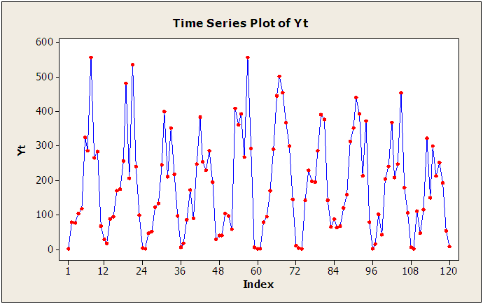 | Figure 1. Raw data plot of the original series  |
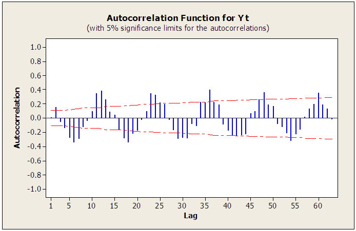 | Figure 2. Autocorrelation plot of the original series  |
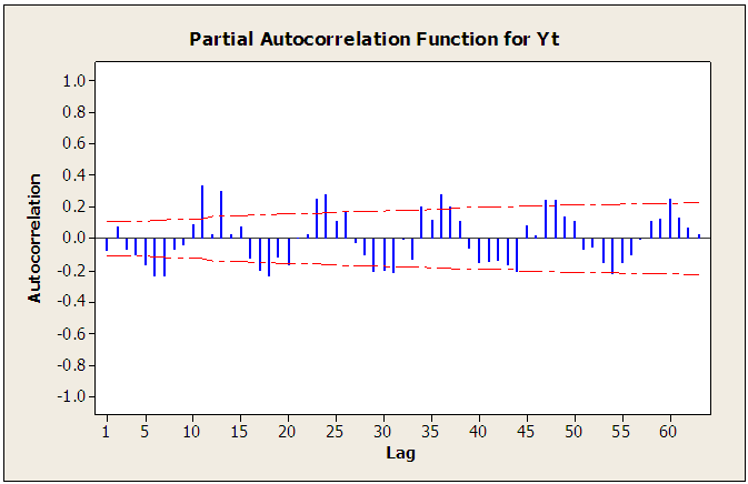 | Figure 3. Partial Autocorrelation plot of the original series  |
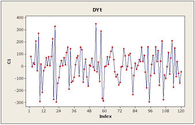 | Figure 4. Plot of the differenced series  |
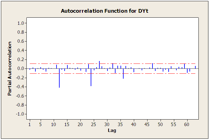 | Figure 5. Autocorrelation plot of the differenced series  |
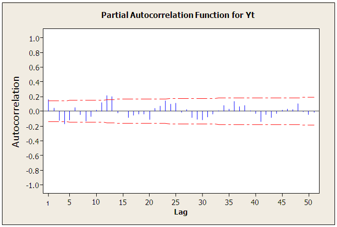 | Figure 6. Partial Autocorrelation plot of the differenced series  |
Substituting the SARIMA coefficient provided by the Minitab software in table 1, we have: | (5) |
Table 1. SARIMA Coefficients
 |
| |
|
The residual autocorrelation function of the above model is displayed in figure 7. As clearly seen, there are some significant spikes which are out of the two boundary lines. This is an indication that the residuals  are correlated and do not follow white noise process. Hence, the model (5) is inadequate.
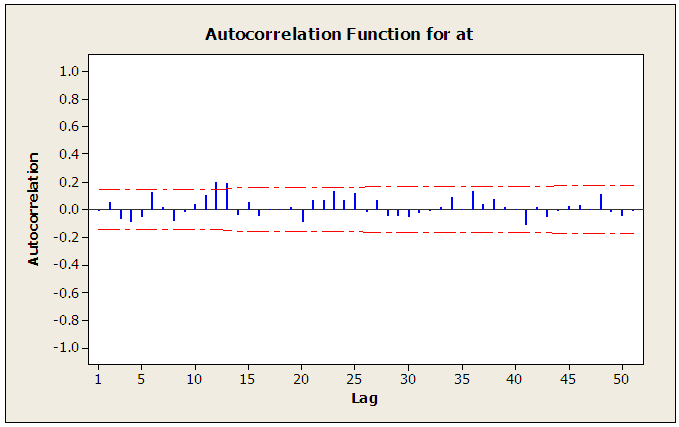 | Figure 7. Autocorrelation plot of the residual series  |
4.1. The Residual ARMA Approach
In this approach, the correlated residuals  are subjected to the Box and Jenkins (1976) ARMA methods. The autocorrelation function (ACF) of the
  series displays a sinusoidal pattern (see figure 7) while its partial autocorrelation function (PACF) cut off after lag 1 (see figure 8). Thus the identified model is ARMA (1, 0) which can be expressed as
 | (6) |
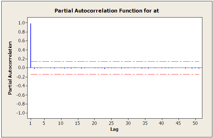 | Figure 8. Partial Autocorrelation plot of the residual series  |
As described in the methodology, equation (6) is substituted in equation (4) to give: | (7) |
which yields | (8) |
The autocorrelation function of the residual  is displayed in figure 9. Clearly, there is no significant autocorrelation of the residuals since all the autocorrelations are within the limits
  (shown by the two lines in figure 9;
  is the sample size). Hence, the fitted model (8) is adequate.
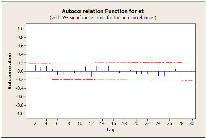 | Figure 9. Autocorrelation plot of the residual series  |
5. Discussion and Conclusions
Usually, in time series modelling; if the fitted model is inadequate, it is replaced by an entirely new model that best fit the data. However, it may be difficult to search for the appropriate model through the usual process and sometimes may be time consuming. The proposed method in this work is advantageous in the sense that it is cheap, simple and less time consuming. Rather than trying or searching for alternative models {as proposed by [2]}, this method utilizes the residuals obtained from the first fitted model to build the final model that best fit the data. As illustrated above, the method has yielded dependable results. It is therefore believed that this proposal has offered another possibility of modelling time series processes.
References
| [1] | Box, G.E.P. and Jenkins, G.M. (1976). Time Series Analysis; forecasting and control. Holdenday Inc., San Francisco, California. ISBN: 0-8162-1104-3. |
| [2] | Box, G.E.P., Jenkins, G.M. and Reinsel, G.C. (2008). Time Series Analysis; forecasting and control. Fourth Edition. A John Wiley & Sons, Inc., Hoboken, New Jersey. ISBN: 978-0- 470-27284-8 (cloth). QA 280.B67 2008. 519.5’5-dc22. |
| [3] | John, A.D., David, F.F., Turkur, S.M., Kellie, C.W. and Donald, E.K. (2007). New ARIMA Models for seasonal time series and their application to seasonal adjustment and forecasting. Journal of Applied Statistics. Vol. 6, No. 7, pp. 33-39. |
| [4] | Kirby, H., Dougherty, M. and Watson, S. (1997). ‘’Should we use neural networks or statistical models for short term motorway traffic forecasting?’’ International Journal of Forecasting; 13(1), 43-50. |
| [5] | Norizon, M., Maizah, H.A., Zuhaimy, I. and Suhartono (2010). Double SARIMA model for forecasting load demand. MATIMATIKA, 2010, vol. 26, No. 2, pp. 217-231. |
| [6] | Tea, B. and Maja, M. (2015). Modelling international tourism demand using seasonal ARIMA models. Tourism and Hospitality Management Vol. 21, No. 1, pp. 19-31. |
| [7] | Williams, B.M. and Hoel, L.A. (2003). Modelling and forecasting vehicular traffic flow as seasonal ARIMA process: Theoretical basis and empirical results. Journal of Transportation En-gineering © ASCE. Vol. 6, No. 664. DOI: 10.1061/(ASCE) 0733-947X (2003) 129: 6 (664). |


 obtained were found to be correlated. This indicated the inadequacy of the model. The correlated residual series were modelled separately using Box and Jenkins autoregressive moving average (ARMA) methods. The resulting residual model was added to the SARIMA component to obtain a new model. The new model was re-fitted to the data and the residuals
  obtained were found to be uncorrelated; confirming the adequacy of the new model.
 is said to be a white noise process with mean 0 and variance
  written
  if it is a sequence of uncorrelated random variables from a fixed distribution.

 can be expressed as


 is the time series at period
  is the (residuals) white noise process,
  represents the backshift operator,
  is the season,
  is the order of non-seasonal autoregressive components,
 the order of seasonal autoregressive components,
  is the order of non-seasonal differencing,
 the order of seasonal differencing,
  is the order of non-seasonal moving average component,
 is the order of seasonal moving average component.
 in (1) does not follow a white noise process; this approach proposes that the residuals
  be modelled separately by ARMA methods and the result be added to the SARIMA part. That is,
 is the (residuals) white noise process obtained from modelling
  separately using the ARMA methods. Equation (2) implies that
 is the moving average operator from the
  series.
 is the autoregressive operator from the
  series.Putting (3) in (1), we obtain
 The residuals obtained by this approach are found to be uncorrelated and follow a white noise process as will be demonstrated in the next section.
  . Figure 1 clearly shows that the series is not stationary; and differencing transformation was applied to obtain stationarity (see figure 4). The ACF plot of the stationary
  series in figure 5 decays exponentially to zero at the seasonal lags 12, 24, 36,… ; and alternate at the non-seasonal lags. However, the PACF of
  (see figure 6) cut off after lag 12 at the seasonal lags and after lag 1 at the non-seasonal lags. The behaviours of the ACF and PACF suggest that the appropriate model for the series is SARIMA (1,1,0)(1,0,0)12. Applying equation (1), the model can be expressed as:
 which gives


 are correlated and do not follow white noise process. Hence, the model (5) is inadequate.

 are subjected to the Box and Jenkins (1976) ARMA methods. The autocorrelation function (ACF) of the
  series displays a sinusoidal pattern (see figure 7) while its partial autocorrelation function (PACF) cut off after lag 1 (see figure 8). Thus the identified model is ARMA (1, 0) which can be expressed as


 is displayed in figure 9. Clearly, there is no significant autocorrelation of the residuals since all the autocorrelations are within the limits
  (shown by the two lines in figure 9;
  is the sample size). Hence, the fitted model (8) is adequate.

 Abstract
 Reference
 Full-Text PDF
 Full-text HTML