Basanta Dhakal
Research Scholar, Central Department of Statistics, Tribhuvan University, Kathmandu, Nepal
Correspondence to: Basanta Dhakal , Research Scholar, Central Department of Statistics, Tribhuvan University, Kathmandu, Nepal.
| Email: |  |
Copyright © 2016 Scientific & Academic Publishing. All Rights Reserved.
This work is licensed under the Creative Commons Attribution International License (CC BY).
http://creativecommons.org/licenses/by/4.0/

Abstract
Tourism being one of the major foreign exchange earnings and job providing sectors is a growing service industry in Nepal. The objective of this paper is to investigate Nepal's foreign exchange earnings through tourism with an analysis of the international tourists’ arrival and the duration they spent in Nepal. The researcher has used annual time series data (1991-2014) provided by Ministry of Tourism and Civil Aviation Nepal to analyze the foreign exchange earnings from tourism by using Johansen test of co-integration and Granger Causality. The empirical result from the co-integration analysis concludes that there exists long-run relationship among the foreign exchange earnings from tourism, number of international tourists, and average length of tourist stay. The findings from Granger causality analysis show the existence of unidirectional causality from number of international tourists to foreign exchange earnings through tourism, and average length of stay to foreign exchange earnings. Similarly, bidirectional causality is also found between number of international tourist and their length of stay. This study posits that the increased tourists’ length of stay and number of international tourists’ arrival will lead to rise in foreign exchange earnings, which has multiplier effect by increasing number of places of amenities for the tourists.
Keywords:
Causality, Length of stay, Tourist arrivals
Cite this paper: Basanta Dhakal , Analyzing Nepal’s Foreign Exchange Earnings from Tourism using Co-integration and Causality Analysis, American Journal of Mathematics and Statistics, Vol. 6 No. 6, 2016, pp. 227-232. doi: 10.5923/j.ajms.20160606.01.
1. Introduction
Foreign exchange earnings are the monetary gains obtained by selling goods and services or by exchanging currencies in global market. “Tourism industry earns the gross revenue and foreign exchange earnings which play an important role in economic development of a nation. It is therefore, a generator of foreign exchange at the national level and also fast-growing industry in the global economy [1]”. Tourism is one of the productive business activities directed for the production of the goods and services. It provides goods and services to visitors, and employment opportunities to the local people. It increases the foreign exchange earnings generating employment opportunities.Nepal has huge potentiality for the tourism development. In this context, the government of Nepal itself has tried to invest for the tourism infrastructure development and institutional buildings encouraging the private sectors to invest by various policy interventions. Tourism not only contributes to the economic growth through multiplier effects but also supplies the foreign currency required for major investment, which is used to import much needed modern technology, machines/equipments and management skills. The government, thus, has taken initiation and a lead role so as to invest in the development of tourism facilities and infrastructures which can be used by the other sectors of economy. “Government of Nepal has also received foreign aid from the Asian Development Bank for the up-gradation of Tribhuvan International Airport and other tourism facilities and infrastructures; the high requirements of capital for the development of tourism infrastructures/facilities force the government in the destination to seek foreign capital. Some standard hotels and tourist enterprises are run by foreigners under foreign direct private investment [2]”. Various empirical papers analyze the tourisms’ contribution to the economic growth of different countries by using error correction model and Granger causality. For examples: Balaguer and Cantavilla [3] investigated the direction of relationship between tourism and economic growth using error correction model and found that the long run causality goes from tourism to economic growth of Spain. Dritsakis [4] for Greece and Durbarry [5] for Mauritius found bidirectional causality between tourism development and economic growth using error correction model. Gunduz and Hatemi-J [6] located unidirectional causality from tourism to Turkeys’ economic growth using leveraged bootstrap causality test for the period of 1963-2002. On the other hand, Ongan and Demiroz [7] suggested bidirectional causality between international tourism and economic growth in Turkey for the period of 1980Q1- 2004Q2 using Granger causality test. Oh [8] got a relation from only economic growth to tourism development for Korea using Granger causality test. Kim et al. [9] found out the bidirectional causality between tourism expansion and economic growth in Taiwan for the period of 1971-2003 using Granger causality. Lee and Chang [10] found unidirectional causality relationship from tourism development to economic growth in Organization and Economic Co-operation and Development (OECD) countries and bidirectional relationship in non-OECD countries, but only weak relationship in Asia for the period of 1990-2002. Kreishan [11] found that there exists unidirectional relationship from tourism development to economic growth of Jordan for the period of 1970-2009 using Granger causality. Georgantopoulos [12] explained relationship between tourism expansion and economic development during the period of 1988-2011 for India and found out bidirectional strong causal links between economic growth and leisure travel and tourism expenditures. All of the above mentioned researchers found that tourism provides significant contribution to national income along with generating employment in the service industries of economy such as hotel, restaurant, travelling, handicraft etc. Tourism is one of the main sources of foreign exchange earnings and major job provider as it is one of rapidly growing service sectors in Nepal. Giving the highest premium to this reality, this study has attempted to investigate the long-run and short-run causal relationship between number of international tourists arriving in Nepal and their length of stay in tandem with foreign exchange earnings from tourism (in USD) using co-integration and causality analysis.
2. Methods
The annual data from the period of 1991 to 2014 is taken from Nepal tourism Statistics available in Ministry of Tourism and Civil Aviation (MOTCA) [13]. Data set is converted into logarithmic return form in order to achieve the long-run and short-run relationship and to make statistical test procedure valid. The statistical analysis is performed using STATA 9.0, College Station, Texas, USA. In order to examine the relationship among foreign exchange from tourism (EARN), average length of stay (AVLS) and number of international tourists’ arrival in Nepal (TOUR), the following model is specified. | (1) |
Where EARN is dependent variable and AVLS and TOUR are explanatory variables. Several tools and techniques have been used for statistical analysis. First of all, Augmented Dickey Fuller [14], [15] test has been used to test the stationary or non-stationary of the individual series of data.  | (2) |
Where Δ is the difference operator, the ADF regression tests for the existence of unit root of Yt namely in the logarithm of all model variable at time t, variable ΔYt-1 expresses the first difference with p lags and final εt is the variable that adjust the errors of autocorrelation. The coefficients δo, δ1, δ2 and αi are being estimated.To determine the correct specification of the unit root test, Akaike Information Criteria (AIC) or Schwartz Bayesian Information Criteria (SBIC) has been used for selecting lag length in various optimal specification of equations [16].The proper order of the model is determined by computing co-integrating equation over a selected grid of values of the number of lags p and finding that value of p at which the AIC or SBIC attain the minimum. AIC and SBIC has been computed using equation (3) and (4). | (3) |
 | (4) |
Where n is number of parameters estimated and T is number of usable variables To determine the most stationary linear combination of the time series variables, Johansen Co-integration test [17] has been used and then the Johansen VECM framework can be expressed as: | (5) |
Where δ is the kx1 vector of parameter that implies the quadratic time trend. Similarly, β is coefficient of co-integrating equation and α is the adjustment coefficient. V is a kx1 vector of parameters. Johansen‘s approach derives two likelihood estimators for determining the number of co-integration vectors: a trace test and a maximum Eigen value test.The Maximum Eigen value statistic tests the null hypothesis of r co-integrating relations against the alternative of r+1 co-integrating relations for r=0,1,2………n-1. It is computed as | (6) |
Where λ is the maximum Eigen value and T is the sample size. Trace statistics investigates the null hypothesis of r co-integrating relations against the alternative of n co-integrating relations, where n is the number of variables in the system for r=0,1,2……..n-1. It is computed through the use of the following formula: | (7) |
In this test, the null hypothesis of r co-integrating vectors is tested against the alternative hypothesis of r+1 co-integrating vectors.Vector Error Correction Model (VECM) has been used to test the long run relationship between target variables and explanatory variables. For this purpose, consider a Vector Autoregressive (VAR) with lag order p which is expressed as  | (8) |
Where Yt is a Kx1 vector of variable, V is a kx1 vector of parameters, AI, A2, A3 ,…………..Ap are k x k matrices of parameters, and εt is a kx1 vector of disturbances having mean 0 and sum of covariance matrix is identically and independently distributed normally over a time period. Any Vector Autoregressive (VAR) Model can be rewritten as Vector Error Correction Model (VECM) by using some algebra, which gives long-run and short-rum information between dependent and independent variables [18].  | (9) |
Where  and
and 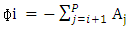 Where Yt is a Kx1 vector of variable, V is a kx1 vector of parameters, AI, A2, A3 ,…………..Ap are k x k matrices of parameters, and εt is a kx1 vector of disturbances having mean 0 and sum of covariance matrix is identically and independently distributed (i.i.d.) normal over a time.If co-integration has been detected between the series, there exists a long term equilibrium relationship between them, and VECM is applied in order to evaluate the short run properties of the co-integrated series. In case of no co-integration, VECM is no longer required and directly proceeds to Granger causality test to establish causal links between variables [19].According to Granger [20], if a scalar Y can help to estimate another scalar X, then we say that Y Granger causes X. If Y causes X and X does not cause Y, it is said that unidirectional causality exists from Y to X. if Y does not cause X and X does not cause Y, then X and Y are statistically independent. If Y causes X and X causes Y, it is said that bidirectional causality exists between X and Y. To implement the Granger causality analysis, a particular autoregressive lag length k(or p) is assumed and model (10) and (11) are estimated:
  | (10) |
 | (11) |
In the model, t denotes time periods, μ is a white noise error and λ is constant parameters.Lagrange-Multiplier (L-M) test [21] has been used to test for autocorrelation as well as test for stability of the model. The formula for L-M test statistic of lag p is expressed as: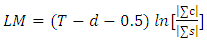 | (12) |
Where T is the number of observations and d is the number of coefficients estimated in augmented VAR; ∑c is the maximum likelihood estimate of variance-covariance matrix (∑) of the disturbances; ∑s is the maximum likelihood estimate of ∑ from augmented vector autoregressive [22]. Finally, Jarque-Bera (J-B) test [23] has been applied for examining the normality of disturbances distribution which is based on the fact that skewness and kurtosis of normal distribution equal to zero.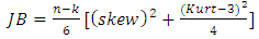 | (13) |
Where n is number of observations and k is number of regressors.
3. Results and Discussions
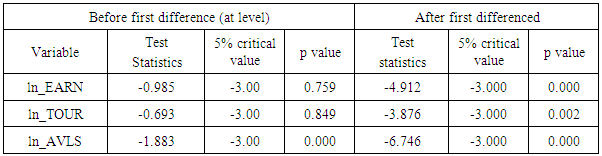
The first step in co-integration analysis is to test the unit roots in each variable. For this purpose, Augmented Dickey Fuller test is applied on EARN, TOUR and AVLS. Table 1. Results of Augmented Dickey Fuller Test
 |
| |
|
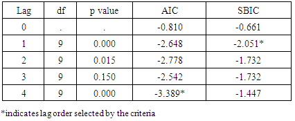
The results of the ADF test in Table 1 indicate that the series of variables such as EARN and TOUR are not stationary in their level (before the first difference) but they all are stationary after the first difference (p value <0.05). It means that all variables are free from unit roots after the first difference. This implies that all the variables in the series are integrated of order one. For getting optimal lag length for co-integrating analysis, two criteria: Akaike Information Criteria (AIC) and Schwarz Bayesian Information Criteria (SBIC) have been adopted as shown in Table 2. Table 2. Results of Lag-order Selection Criteria
 |
| |
|
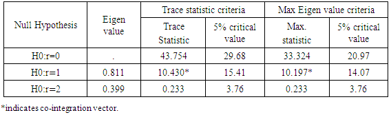
Table 2 shows that AIC is minimum at 4 lag length and SBIC is minimum at 1 lag length. It means that SBIC suggested there is 1 optimal lag length, while AIC indicated 4 as optimal lag length. But in this study of series (EARN, TOUR & AVLS) for co-integration analysis, 4 lag length has been adopted because 1 lag length could not be found the co-integrating vector under both trace and maximum Eigen value statistics (Table 3) while at lag length 4 could be found one co-integrating vector under both these statistics. Co-integration relationship among EARN, TOUR and AVLS has been investigated using the Johansen technique. Table 3 reports the results of co-integration test based on Johansen’s Maximum likelihood method. Both trace statistic and maximum Eigen value statistic indicate that there is at least one co-integrating vector among EARN, TOUR and AVLS. It can reject the null hypothesis of no co-integrating vector against under both test statistics at 5% level of significant. It also can not reject the null hypothesis of at most one co-integration vector against the alternative hypothesis of two co-integrating vectors for both trace and max Eigen value test statistics. Consequently, it can conclude that there is one co-integrating relationship among EARN, TOUR and AVLS. This implies the EARN, TOUR and AVLS establish a long run relationship. It obviously opens the system for applying VECM and the summary of relationship between EARN, TOUR and AVLS under VECM can be displayed in Table 4.Table 3. Results of Johansen Test of Co-integration
 |
| |
|
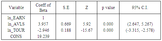
Table 4. Results of Co-integration Equation
 |
| |
|
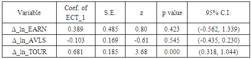
The long run relationship among foreign exchange earnings from tourism, number of international tourists and their average length of stay for one co-integrating vector for Nepal in the period 1991-2014 are displayed below (standard errors are displayed in parenthesis) 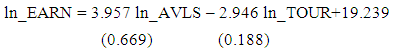 The co-integration equation has been normalized in logarithmic returns form in order to get meaning of coefficients of elasticity i.e. if all variables are logarithmic; it may be easy to interpret the coefficients in terms of elasticity. So it may say increasing EARN by 100% produces an increment of almost 395.69% of AVLS. Similarly increasing EARN by 100% produces an impact of almost 294.62% of TOUR. Thus EARN elasticity with respect to AVLS is more elastic as compared to EARN elasticity with respect to TOUR.The large absolute value of the coefficient of error correction terms (ECT) shows fast speed of adjustment towards equilibrium while low absolute values are indicating of slow speed of adjustment. Table 5 indicates TOUR has fast speed of adjustment towards equilibrium and AVLS has slow speed of adjustment. The coefficient of error correction term of EARN has positive sign and it is statistically insignificant at 5% level. It implies that the system divergence from equilibrium but unstable due to the any disturbance in the system. The coefficient of error correction term of AVLS carries negative sign but it is insignificant at 5% level. It depicts that the system convergence towards equilibrium but unstable in case of any disturbance in the system. The coefficient of error correction term of TOUR is positive and statistically significant at 5% level. It implies that the TOUR divergence from the equilibrium and stable due to any disturbance in the system.
Table 5. Results of Coefficient of Error Correction Terms
 |
| |
|
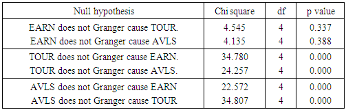
In order to analyze bidirectional and unidirectional causal relationship among EARN, TOUR and AVLS, Granger Casualty Wald test is used for the test of significance of the lagged variables in that equation (Table 6).Table 6. Results of Granger Causality Wald Test
 |
| |
|
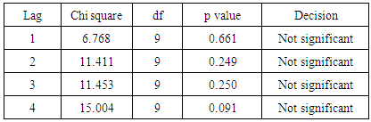
Table 6 reports the results causal relationship among the variable EARN, TOUR and AVLS. It shows that TOUR Granger causes AVLS and AVLS also Granger causes TOUR. So bidirectional Granger causality exists between TOUR and AVLS. It signifies the past values of TOUR have predictive ability to determine the present value of AVLS and vice versa. Similarly, TOUR Granger causes EARN but EARN does not Granger cause TOUR. So, unidirectional Granger causality exists from TOUR to EARN. In addition, AVLS Granger Causes EARN but EARN does not Granger cause AVLS. So, unidirectional Granger causality exists from AVLS to EARN. It implies that the past values of TOUR and AVLS have predictive ability to determine the present value of EARN.The stability of the Model has been assessed through the L-M test for autocorrelation, and the results are presented in Table 7.Table 7. Results of L- M Test of Autocorrelation
 |
| |
|
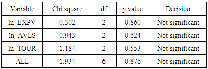
Table 7 shows that Lagrange –Multiplier test concludes it cannot reject the null hypothesis of no residual autocorrelation at lag order 1 through 4, so there is no evidence to contradict the validity of the model. Finally, the test of normality of disturbances distribution in the series of the variables has also been evaluated by Jarque-Bera test (Table 8). Table 8. Results of Jarque –Bera Test for Normality Distributed Disturbances
 |
| |
|
Table 8 shows that Jarque-Bera test concludes that the disturbances are distributed normally.
4. Conclusions
The Johansen test of co-integration indicates that there exists one co-integrated vector among the variables. Meaning that there exists long-run relationship among the variables such as EARN, TOUR and AVLS under 4 lag of length. The long-run relationship based on vector error correction model has indicated that coefficient of elasticity of foreign exchange earnings from tourism vis-à-vis average length of stay is relatively elastic as compared to foreign exchange earnings and the number of international tourists’ arrival in Nepal. The results of Granger causality test depicts that the unidirectional causal relationship between number of international tourists arrival and foreign exchange earnings from tourism. Similarly, there is unidirectional causality from average length of stay of tourists to foreign exchange earnings from tourism. In addition, there exists bidirectional causal relationship between international tourists’ arrival in Nepal and their average length of stay. It indicates that the length of stay of tourist increases foreign exchange earnings and the increased number of international tourist plays the positive role to expand their length of stay by increasing amenities. It clarifies that expansion of foreign exchange earnings will lead to the expansion of tourists’ length of stay on the one hand and it further incorporates to attract number of international tourists to Nepal. Focusing on foreign exchange earnings from tourism activities in Nepal, this study offers that more efforts should be concentrated on upgrading tourism related facilities such as hotel and restaurants, tourist resorts, entertainment centers, transportation services, sales outlet of curios, handicraft, amusement parks, cultural activities etc for increasing number of international tourists and their length of stay.
ACKNOWLEDGEMENTS
I am very thankful to Pro. Dr. Azaya Bikram Sthapit and Pro. Dr. Shankar Prasad Khanal, whose suggestions led to conduct of this study.
References
| [1] | Gill, N. and, Singh, R.P. 2013. “Socio-economic impact assessment of tourism in Pithoragarh district, Uttarakhand” International Journal of Advancement in Remote Sensing, GIS and Geography, 1:1-7. |
| [2] | Paudyal, S.R. 2012. “Does tourism really matter for economic growth? Evidence from Nepal” Nepal Rastra Bank Economic Review, 24:58-89. |
| [3] | Balaguer, J. and Catavella-Jorda, M. 2002. “Tourism as a long run economic growth factor: the Spanish case” Applied Economics, 34(7): 877-884. |
| [4] | Dritsakis, N. 2004. “Tourism as a long-run economic growth factor: an empirical investigation for Greece using causality analysis” Tourism Economics, 10(3):305-316. |
| [5] | Durbarry, R. 2004. ”Tourism and economic growth: The case of Mauritius” Tourism Economics, 10 (4):389-401. |
| [6] | Gunduz, L. and Hatemi-J, A. 2005. “Is the tourism-led growth hypothesis valid for Turkey?” Applied Economic Letters, 12(8): 499-504. |
| [7] | Ongan, S. and Demiroz, D. M. 2005. “The contribution of Tourism to the long-run Turkish economic growth” Journal of Economics, 53 (9):880-894. |
| [8] | Oh, C. 2005. “The contribution of tourism development to economic growth in the Korean economy” Tourism Management, 26(1): 39-44. |
| [9] | Kim, H.J., Chen, M. and Jan, S. 2006. “Tourism expansion and economic development: The case of Taiwan” Tourism Management, 27:925-933. |
| [10] | Lee, C. and Chang, C. 2008. “Tourism development and economic growth: A closer look panels” Tourism Management, 29,180-192. |
| [11] | Kreishan, F. 2011. “Time-series evidence for tourism-led growth hypothesis: A case study of Jordan” International Management Review, 7(1): 89-93. |
| [12] | Geogantopouls, A.G. 2013. “Tourism expansion and economic development: VAR/VECM analysis and forecasts for the case of India”. Asian Economic and Financial Review, 3(4): 464-482. |
| [13] | MOTCA 2009-2014. Ministry of Tourism and Civil Aviation. Nepal Tourism Statistics. Government of Nepal. |
| [14] | Dickey, D. and Fuller W. 1979. “Distribution of the estimators for autoregressive time series with a unit root” Journal of the American Statistical Association, 74(366): 427-431. |
| [15] | Dickey, D. and Fuller W. 1981. “Likelihood ratio statistics for autoregressive time Series with a unit root” Econometrica, 49: 1057-1072. |
| [16] | Mukhtar, T. and Rasheed, S. 2010. “Testing long run relationship between exports and imports: Evidence from Pakistan” Journal of Economic Cooperation and Development, 31: 41-58. |
| [17] | Johansen, S. 1988. “Statistical analysis of co-integration vectors” Journal of Economic Dynamics and Control, 12:231-254. |
| [18] | Johansen, S. 1995. Likelihood- based inference in co-integrated vector autoregressive model. Oxford: Oxford University Press. |
| [19] | Becketti, S. 2013. Introduction to time series using stata. College Station’s: Stata Press. |
| [20] | Granger, C.W.C. 1969. “Investigating causal relations by econometric models and cross-spectral methods”. Econometrica, 37: 424-438. |
| [21] | Breusch, T.S. and Pagan, A.R. 1980. “The Lagrange multiplier test and its applications to model specification in econometrics” Review of Economic Studies, 47:239-253. |
| [22] | Davidson, R. and Mackinnon, J.G. 1993. Estimation and Inference in Econometrics, Oxford: Oxford University Press. |
| [23] | Jarque, C.M. and Bera, A. K. 1987. “A test for normality of observations and regression residuals” International Statistical Review, 55:163-172. |

 Abstract
 Reference
 Full-Text PDF
 Full-text HTML