Md. Tarek Hossain, Md. Shah Alam
Department of Physics, Shahjalal University of Science and Technology, Sylhet, Bangladesh
Correspondence to: Md. Tarek Hossain, Department of Physics, Shahjalal University of Science and Technology, Sylhet, Bangladesh.
| Email: |  |
Copyright © 2016 Scientific & Academic Publishing. All Rights Reserved.
This work is licensed under the Creative Commons Attribution International License (CC BY).
http://creativecommons.org/licenses/by/4.0/

Abstract
The Lorentz transformation can be explained in two ways i.e. the special Lorentz transformation and most general Lorentz transformation. The length contraction, time dilation and velocity addition formulas for the special and most general Lorentz transformations are clearly explained. The variation of mass due to the relativistic velocity has also explained. Using above mentioned parameters we have derived the formulas of the transformation of orbital angular momentum and spin angular momentum for special Lorentz transformation. We have calculated the values of orbital angular momentum for rest and moving observers. The values of orbital angular momentum have plotted for the different velocities of the moving observers.
Keywords:
Special Lorentz transformation, Most general Lorentz transformation, Angular momentum, Length contraction, Velocity addition formula
Cite this paper: Md. Tarek Hossain, Md. Shah Alam, Transformation of Orbital Angular Momentum and Spin Angular Momentum, American Journal of Mathematics and Statistics, Vol. 6 No. 5, 2016, pp. 213-226. doi: 10.5923/j.ajms.20160605.03.
1. Introduction
1.1. Lorentz Ttransformation
The transformation which relates the observations of position and time made by the two observers in two different inertial frames is known as Lorentz transformation.
1.2. Special Lorentz Transformation
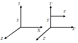 | Figure 1. The frame S is at rest and the frame S′ is moving with respect to S with uniform velocity v along x-axis |
Let us consider two inertial frame of references S and S′ where the frame S is at rest and the frame S′ is moving along x-axis with velocity v with respect to S frame. The space and time coordinates of S and S′ are (x,y,z,t) and (x′,y′,z′,t′) respectively. The relation between the coordinates of S and S′, which is called special Lorentz Transformation, can be written as [1, 3-5]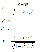 | (1) |
1.3. Most General Lorentz Transformation
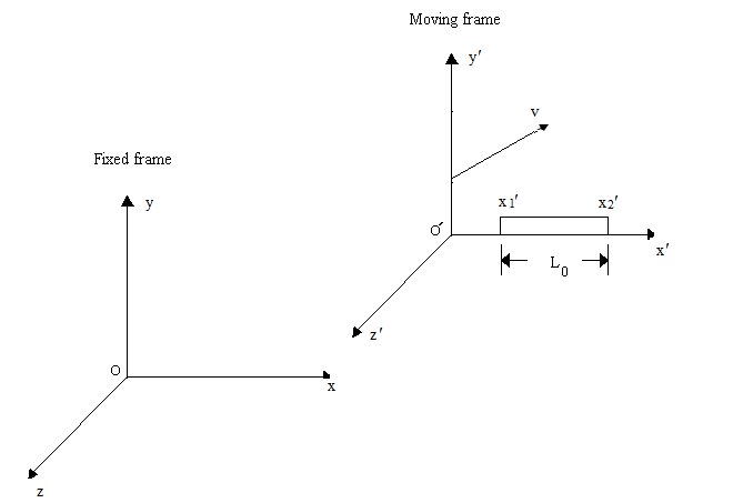
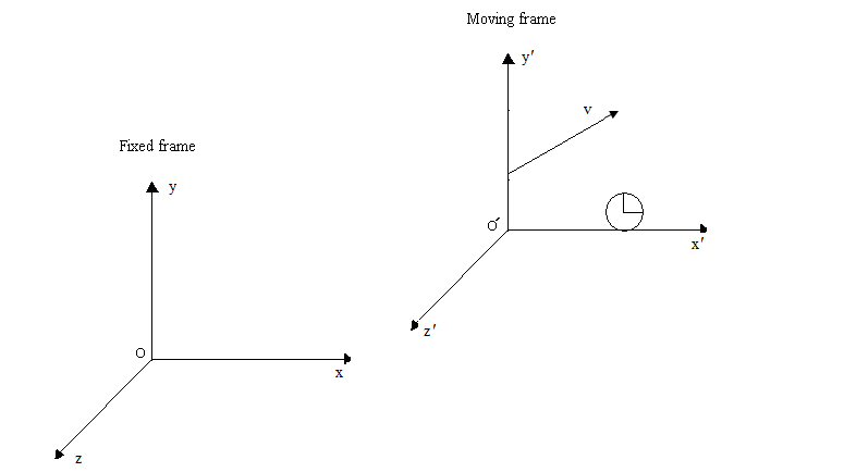
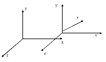 | Figure 2. The frame S is at rest and the frame S′ is moving with respect to S with uniform velocity v along any arbitrary direction |
When the velocity  of S′ with respect to the S is not along x-axis i.e. the velocity
  has three components vx, vy and vz then the relation between the coordinates of S and S′, which is called most general Lorentz transformation, can be written as [2-5]
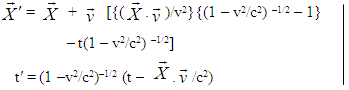 | (2) |
Here  and
and  is the space part of the S and S′ frame respectively.
2. Consequence of Lorentz Transformation
2.1. Length Contraction of Special Lorentz Transformation
The length of any object in a moving frame will appear shortened (or contracted) in the direction of motion. The amount of contraction can be calculated from the Lorentz transformation. The length is maximum in the frame in which the object is at rest.If the length L0 = x2′ − x1′ is measured in the moving reference frame and the length L= x2 – x1 is measured in the rest reference then using special Lorentz Transformation. The relation between L and L0 can be written as [1] | (3) |
This is the formula of length contraction for Special Lorentz transformation.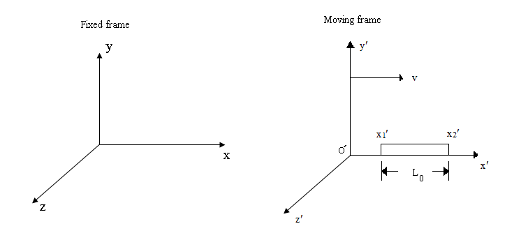 | Figure 3. A frame is at rest and another frame is moving along X-axis with respect to the rest frame. A rod of length L0 is at rest with respect to the moving frame |
 | Figure 4. A frame is at rest and another frame is moving along arbitrary direction with respect to the rest frame. A rod of length L0 is at rest with respect to the moving frame |
2.2. Length Contraction of Most General Lorentz Transformation
Let,  Using Eq. (2), we can write
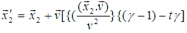 Where,
 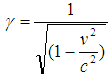 and
and  Therefore,
 | (4) |
(where,  )This is the formula of length contraction for the most general Lorentz transformation. If
  is along the x-axis, then
  We get from Eq. (4)
 or,
or,  This is the same as Eq. (3).
2.3. Time Dilation of Special Lorentz Transformation
A clock in moving frame will be seen to be running slow or “dilated” according to Lorentz transformation. The time will always be shortest as measured in the rest frame. The time measured in which the clock is at rest called the “proper time”.If the time interval T0 = t2′− t1′ is measured in the moving reference frame, than T = t2 − t1 can be calculated using the special Lorentz transformation (Eq. 1). The time measurements made in the moving frame at the same location, so the expression reduces to
 This is the formula of time dilation for the Special Lorentz transformation.
2.4. Time Dilation of Most General Lorentz Transformation
T = t2 − t1 can be calculated using the most general Lorentz transformation. | (5) |
This is the formula of time dilation for the most general Lorentz transformation which is the same as that of the Special Lorentz transformation.
2.5. Relativistic Velocity Addition Formula for Special Lorentz Transformation
Consider two systems S and S′, S be the ground frame and S be the frame of the train, whose speed relative to the ground is v. The passenger’s speed in the S′ is u′. The passenger’s speed u relative to the ground can be written as [1] | (6) |
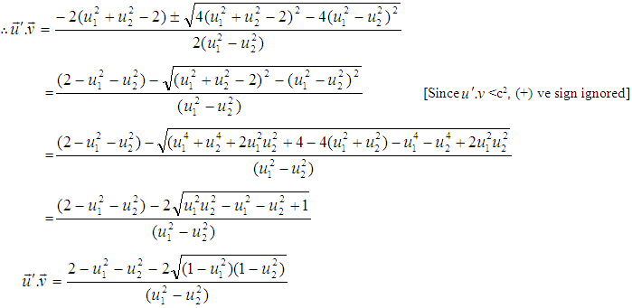
In unit of c, equation (6) can be written as | (7) |
Equation (7) is the relativistic or Einstein velocity addition theorem for special Lorentz transformation.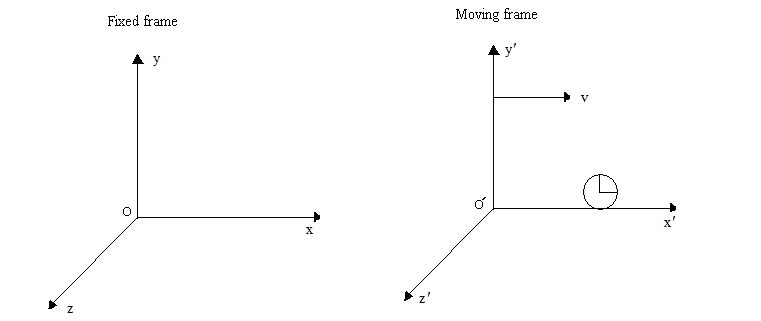 | Figure 5. A frame is at rest and another frame is moving along X-axis with respect to the rest frame. A clock is at rest with respect to the moving frame |
 | Figure 6. A frame is at rest and another frame is moving along arbitrary direction with respect to the rest frame. A clock is at rest with respect to the moving frame |
2.6. Relativistic Velocity Addition Formula for Most General Lorentz Transformation
In this case the relativistic velocity addition theorem can be written as [6]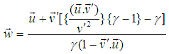 | (8) |
Where  Putting
  , equation (8) takes the form
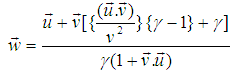 | (9) |
Equation (9) is the relativistic velocity addition theorem for most general Lorentz transformation.
3. Variation of Mass
3.1. Variation of Mass of Special Lorentz Transformation
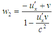
Let there be two systems S and S´, later is moving with velocity v relative to former. Let there be two particles in system S′ traveling with equal and opposite velocities, i.e. u′x and -u′x along (+) ve x′axis. Let these two particles impinge and after impact coalesce into one particle. According to the principle of conservation of momentum, this coalesced particle is at rest with respect to the moving frame. Let m1 & m2 are the masses of the two particles and w1 & w2 are the velocities of the particles as seen from S frame. 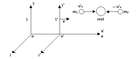 Now for the particle traveling with velocity
  , we have,
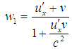 | (10) |
And for the particle traveling with velocity  ,
, | (11) |
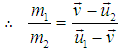
Since after impact the coalesced particle in S′ traveling with velocity v relative to the system S, as the particle is at rest in system S. According to the principle of conservation of momentum as viewed from S,m1 w1 + m2w2 = (m1 + m2) vOr, m1 (w1−v) = m2 (v – w2)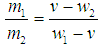 | (12) |
Now putting the values of w1 and w2 in the above equation by considering c = 1,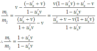 | (13) |
Now squaring (10) & (11) we get, And
And Subtracting these, we get,
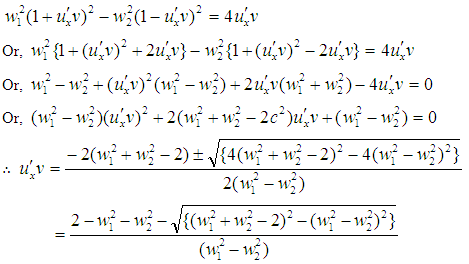 [As
[As  , taking (-) ve sign.]
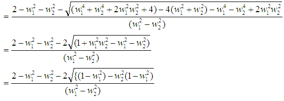 Thus
Thus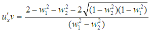 Substituting this value in equation (13) we get,
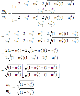 Now if the particle of mass m2 is at rest, then corresponding velocity w2 = 0. We can write with the usual notations m2 = m0 and m1 = m,
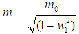 This is the formula for the variation of mass with velocity in special Lorentz Transformation. Thus from the above formula it is clear that the mass of a body increases with increase of velocity.
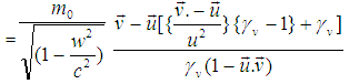
3.2. Variation of Mass of Most General Lorentz Transformation
Now we attempt to find out the variation of mass with velocity in the case of most general Lorentz transformation. Consider two inertial frames S and S′. The later is moving with velocity v in the arbitrary direction relative to the former. Here v has three components. Let us now consider two particles of masses m1 and m2 observed from the frame S. The particles moving with equal and opposite velocity, i.e.  and
and  observed from the frame S´ and they are attempted to impinge. The masses of the particles are equal measured from the frame S′. After impact they coalesced into one particle and become rest relative to the frame S′. Let
  and
and  be the velocity of the particles viewed from the frame S. It should be noted that after impact the coalesced particle moving with the frame velocity (S′) with respect to the rest frame S.
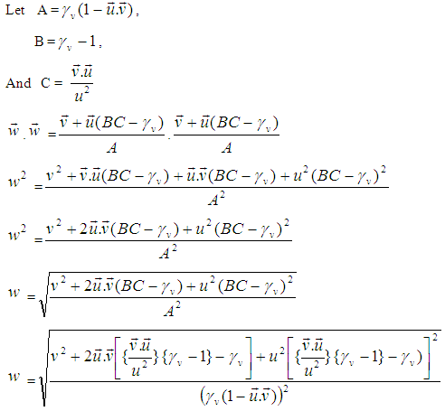
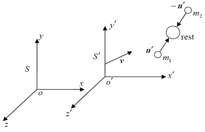 Let us consider c = 1;According to the velocity addition rule of most general Lorentz transformation (equation 13), the velocity of the particle of mass m1 observed from the frame S is,
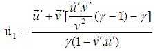 | (14) |
In fact  is the velocity of the S frame relative to the S′ frame. In terms of
  equation (14) can be written as,
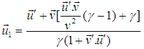 | (15) |
Now the velocity of the particle of m2 observed from the frame S is,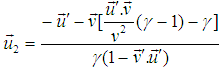 | (16) |
Let m1 and m2 be the masses of the particles moving with velocity  and
and  . Now according to the principle of conservation of momentum as viewed from S is,
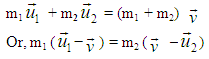
 | (17) |
Now putting the value of  and
and  from equation (15) & (16) in equation (17) we get,
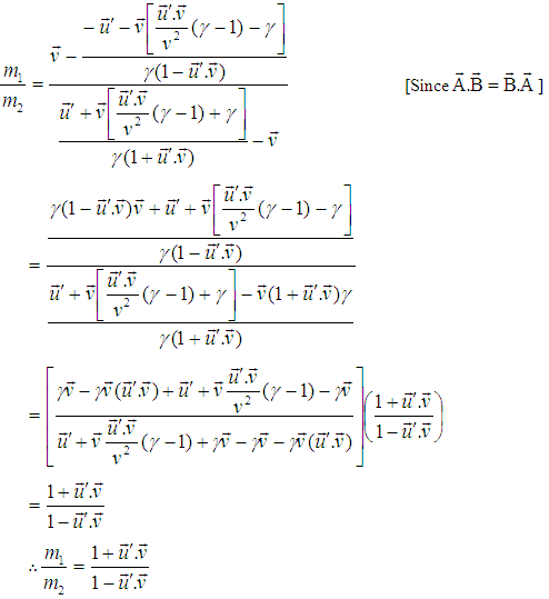 | (18) |
Squaring (15) we have,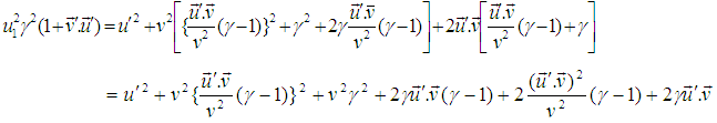 | (19) |
Now Squaring (16) we get,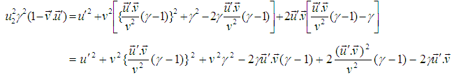 | (20) |
Subtracting (20) from (19) we get,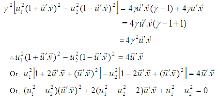
 | (21) |
Putting the value of  from (21), equation (18) becomes,
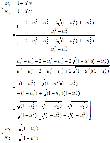 If the particle of mass m2 is at rest,
  = 0 and using the usual notations m2 = m0 and m1 = m, the above equation becomes,
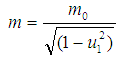 This is the formula for the variation of mass with velocity in most general Lorentz Transformation.
4. Angular Momentum
Let us consider a particle of mass m, which is rotating about a circular path of radius r along anticlockwise direction as shown in the figure 7. At a certain time t, the linear momentum of the particle is,  . The observer O is at rest with respect to the laboratory and the observer O′ is moving with uniform velocity u along x-axis with respect to laboratory [5-6]. According to the definition, the angular momentum of the moving particle observed by the observer O is
  We want to find the angular momentum of the moving particle observed by the observer O′.
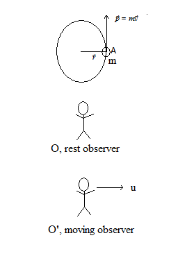 | Figure 7. Rotating particle observing by two observers |
4.1. Angular Momentum Observed by a Rest Observer
For the figure-7, the angular momentum can be written as,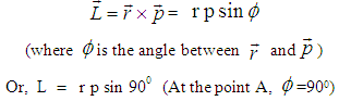 | (22) |
Again, p = m v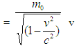 Putting the value of p in equation (22), than we can write
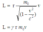 Where,
 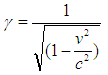 This is the angular momentum formula observed by a rest observer.
4.2. Angular Momentum Observed by a Moving Observer
For figure-7 the velocity of the moving particle with respect to the moving observer the relativistic velocity addition theorem for most general Lorentz transformation equation (9) can be written as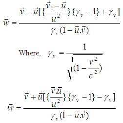 Again,
 Here,
Here,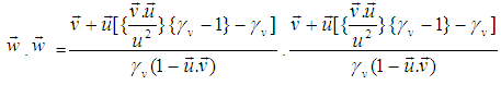
 The angular momentum of the moving particle observed by the moving observer can be written as,
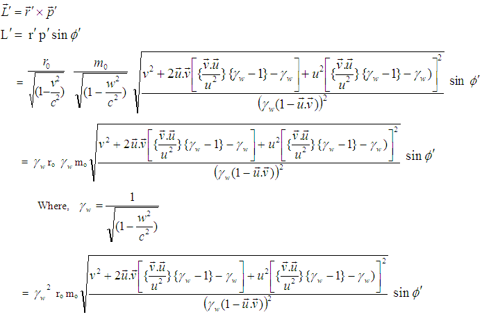 | (23) |
Let the observer O′ is moving with uniform velocity w along x-axis with respect to laboratory. The moving observer O′ observes the angle in rotating particle be  .
.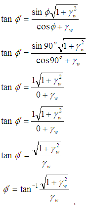 Now putting the value of
  in equation (23),
 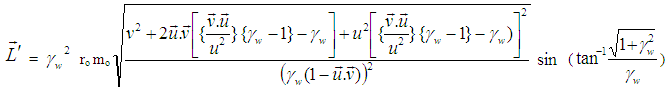 | (24) |
This is the angular momentum equation observed by a moving observer.
4.3. Numerical Calculation
Let us consider the particle is ball. So rest mass of the ball m = 1.00794 Kg and radius a = 5.2910-11 m. We have calculated the angular momentum of the ball for different velocities and presented the values in the following table.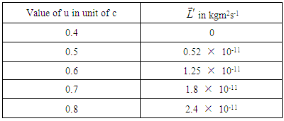 The observer O is at rest with respect to the laboratory and the observer O′ is moving with uniform velocity u along x-axis with respect to laboratory. The change of u angular momentum observed by a moving observer as shown in the figure-8.Using equation (24) the change of the angular momentum observed by a moving observer and rest observer data is shown below.
 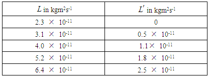 The particle of mass m, which is rotating about a circular path of radius r along anticlockwise direction as shown in the figure – 7. The particle velocity is
  . The change of
  the angular momentum observed by a moving observer and rest observer as shown in the figure-9.
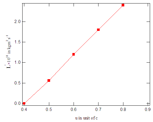 | Figure 8. The change of u angular momentum observed by a moving observer |
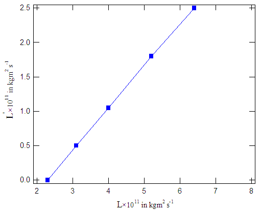 | Figure 9. The change of ν the angular momentum observed by a moving observer and rest observer |
5. Spin Angular Momentum
A solid spherical ball of mass m and radius a is moving about a circular path along anticlockwise direction and it also rotating about its own axis. At a certain time t, the linear momentum of the ball is,  . The observer O is at rest with respect to the laboratory and the observer O′ is moving with uniform velocity u along x-axis with respect to laboratory. The orbital angular momentum of the moving ball observed by the observer O can be written as
  We want to find the spin angular momentum of the moving ball observed by both the observers.
5.1. Spin Angular Momentum Observed by a Rest Observer
Spin is the angular momentum which is associated with a rotating object like a spinning golf ball. The spin angular momentum of such a rigid body can be calculated by integrating over the contributions to the spin angular momentum due to the motion of each of the infinitesimal masses making up the body. The well known result is that the spin angular momentum S can be written as [9] | (25) |
Where I is the moment of inertia and  is its angular velocity of the ball. The moment of inertia is determined by the distribution of mass in the rotating body relative to the axis of rotation. The moment of inertia of the ball can be written as [9]
 | (26) |
The angular velocity of the spinning motion of the ball can be written as, | (27) |
Where T is the time needed for one revolution about own axis of the ball observed by rest observer. Putting the value of I and  from equation (26) and (27) into equation (25) we get,
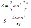 | (28) |
This is the formula of Spin angular momentum of the ball observed by the rest observer O.
5.2. Spin Angular Momentum Observed by a Moving Observer
The Spin angular momentum observed by the moving observer can be written as, | (29) |
Where  is the moment of inertia and
  is its angular velocity of the ball observed by the moving observer. The moment of inertia of the ball observed by the moving observer can be written as,
 | (30) |
The angular velocity of the spinning motion of the ball observed by the moving observer can be written as  | (31) |
Where T' is the time needed for one revolution about own axis observed by moving observer.Putting the value of  and
and  from equation (30) and (31) into equation (29) we get,
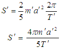 | (32) |
Using equation (3) we can write, 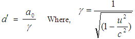 Using equation (5) we can write,
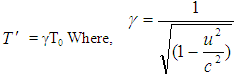 Using equation (18) we can write,
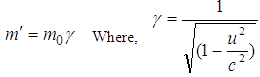 So, equation (30) can be written as,
 | (33) |
This is the formula of Spin angular momentum of the moving ball observed by the moving observer  .
.
6. Conclusions
We have derived the formula for the transformation of orbital angular momentum and spin angular momentum for special Lorentz transformation. We have calculated the value of orbital angular momentum observed from the rest observer and moving observer. The graph of the orbital angular momentum versus velocity of the moving observer has plotted. We have observed that the orbital angular momentum increases due to the increase of the velocity of the observer. The orbital angular momentum observed from the moving observer and rest observer has also plotted. We have also observed that the orbital angular momentum observed from the moving observer is increased due to the increase of angular momentum observed from the rest observer. We have derived the formula of spin angular momentum observed from the rest observer and moving observer. The equation (33) clearly shows that the spin angular momentum decreases due to the increase of the velocity of the observer.
References
| [1] | R. Resnick, Introduction to special relativity, Wiley Eastern limited, 1994. |
| [2] | C. Moller, The Theory of Relativity, Oxford University press, London, 1972. |
| [3] | A. R. Baizid and M. S. Alam, “Applications of different Types of Lorenz Transformations” American Journal of Mathematics and Statistics, 2(5): 153-163, 2012. |
| [4] | A. R. Baizid and M. S. Alam, “Properties of different Types of Lorenz Transformations” American Journal of Mathematics and Statistics, 3(3): 105-123, 2013. |
| [5] | A. R. Baizid and M. S. Alam, “Reciprocal Property of different Types of Lorenz Transformations” International Journal of Reciprocal Symmetry and Theoretical Physics, Volume 1, No 1, 2014. |
| [6] | M.S. Alam, “Study of Mixed Number”, Proc. Pakistan Acad. of Sci, 37(1): 119-122, 2000. |
| [7] | T.A. Nieminen, A.B. Stilgoe, N.R. Heckenberg and H. Rubinsztein-Dunlop “Angular momentum of a strongly focused”, H. 2008. |
| [8] | Barnett, S.M. and Allen L. “Orbital angular momentum and no paraxial light beams”, Opt. Commum, 110, 670-678, 1994. |
| [9] | S. Olszewski, “Electron Spin and Proton Spin in the Hydrogen and Hydrogen-Like Atomic Systems”, Journal of Modern Physics, 5, 2030-2040, 2014. |

 Abstract
 Reference
 Full-Text PDF
 Full-text HTML