I. A. Iwok, A. S. Okpe
Department of Mathematics/Statistics, University of Port-Harcourt, Port-Harcourt, Nigeria
Correspondence to: I. A. Iwok, Department of Mathematics/Statistics, University of Port-Harcourt, Port-Harcourt, Nigeria.
| Email: |  |
Copyright © 2016 Scientific & Academic Publishing. All Rights Reserved.
This work is licensed under the Creative Commons Attribution International License (CC BY).
http://creativecommons.org/licenses/by/4.0/

Abstract
This work compares the performances of univariate and multivariate time series models. Five time series variables from Nigeria’s gross domestic products were used for the comparative study. These series were modelled using both the univariate and multivariate time series framework. The performances of the two methods were evaluated based on the mean error incurred by each approach. The results showed that the univariate linear stationary models perform better than the multivariate models.
Keywords:
Univariate time series, Multivariate process, Stationarity, Stable VAR process, Cross Correlation and VAR order selection
Cite this paper: I. A. Iwok, A. S. Okpe, A Comparative Study between Univariate and Multivariate Linear Stationary Time Series Models, American Journal of Mathematics and Statistics, Vol. 6 No. 5, 2016, pp. 203-212. doi: 10.5923/j.ajms.20160605.02.
1. Introduction
In making choices between alternative courses of action, decision makers often need predictions of some variables of interest. Many of such variables used for predictive purposes are in form of time series. Some variables are economical in nature and the economy partly depends on the interplay of these variables with respect to time. An intrinsic feature of a time series is that, typically, adjacent observations are dependent. The nature of this dependence among observations of a time series is of considerable practical interest. Unlike the analyses of random samples of observations in other aspect of statistics, the analysis of time series is based on the assumption that successive values in the data file represent consecutive measurements taken at equally time intervals. There are two main goals of time series analysis: identification of the nature of the phenomenon represented by the sequence of observations and forecasting (predicting future values of the time series variable). The goals require that the pattern of observed data be identified, described and established so that it can be interpreted and integrated with other data. In data analysis, variables of interest can be univariate or multivariate. In the case of univariate data analysis, the response variable is influenced by only one factor; whereas in the case multivariate, the response variable is influenced by multiple factors. A univariate data is characterized by a single variable. It does not deal with causes or relationships. Its descriptive properties can be identified in some estimates such as central tendency (mean, mode, median), dispersion (range, variance, maximum, minimum, quartile, and standard deviation), the frequency distributions, bar chart, histogram, pie chart, line graph, box and whisker plot. The univariate data analysis is known for its limitation in the determination of relationship between two or more variables, correlations, comparisons, causes, explanations, and contingency between variables. Generally, it does not supply further information on the dependent and independent variables and as such is insufficient in any analysis involving more than one variable. In order to obtain results from such multiple indicator problems, multivariate data analysis is usually employed. This will not only help consider several characteristics in a model but will also bring to light the effect of the extraneous variables (stochastic terms).In the same light, time series analysis can either be univariate or multivariate. The term univariate time series refers to one that consists of single observations recorded sequentially over equal time increments. Unlike other areas of statistics, univariate time series model contains lag values of itself as independent variables. These lag variables can play the role of independent variables as in multiple regression. An example of the univariate time series is the Box et al (2008) Autoregressive Integrated Moving Average (ARIMA) models. On the other hand, multivariate time series model is an extension of the univariate case and involves two or more input variables. It does not limit itself to its past information but also incorporate the past of other variables. Multivariate processes arise when several related time series are observed simultaneously over time, instead of observing a single series as in univariate case. It emerged in quest of studying the interrelationship among time series variables. These relationships are often studied through consideration of the correlation structures among the component series.Both univariate and multivariate time series models are meant for forecasting purposes. There is need, however, to compare the efficiencies of these two models. This is the intent of this work.
2. Literature Review
Henry and Prebo (2005) examined the interrelationships among geophysical variables using the correlation structure of multivariate time series technique. Three of the five variables were found to be interrelated and were modelled as multivariate variables while the remaining two were not put to use in the analytical process. Henry and Prebo (2005) found that the predictions by the multivariate model with only the interrelated variables were quite good. They pointed out that adding of uncorrelated variables in multivariate analysis was not necessary.George (2005) compared the performance of Box-Jenkins univariate model with transfer function models using two economic variables (inflation and Gross domestic product). It was discovered that though univariate analysis could only address one time series variable at a time; it performs far better than the transfer function models in terms of forecasting.Ben et al (2010) proposed a class of nonparametric multivariate model to model nonlinear relationships between input and output time series. The multivariate model was smoothed with unknown functional forms, and the noise was assumed to be a stationary autoregressive moving average process. Modelling the correlation of the noise enabled the multivariate functions to be estimated more efficiently.Oluwatomi et al (2011) made use of vector autoregressive model analysis with impulse response functions and other test to determine the inter relationship between oil price and investment. The result showed that oil price have negligible effect on real GDP. The work further recommended a further assessment using GARCH models.Makridakis and Clay (2012) examined the accuracy of combined forecasts consisting of weighted averages of forecasts from individual univariate time series method. Five different procedures were used to estimate weights and two of the procedures outperformed the others. Both of these procedures relate the weights to reciprocals of sums of squared errors as oppose to basing the weights directly on an estimated covariance matrix of forecast errors obtained in Multivariate method. The research led to a proposed algorithm for estimation of large number of component time series models. It was deduced that if maximum likelihood estimate are wanted for a large model, the algorithm may reduce the computations considerably by supplying good initial estimates. However, in the model identification stage of multivariate time series, the work suggested an estimation of a number of alternative models for which the algorithm was required.Saul et al (2013) applied a multivariate technique to efficiently quantify the frequency response of the system that generated respiratory sinus arrhythmia at broad range physiologically important frequencies. The technique presented sensitively identifies even the subtle changes in autonomic balance that occur with change in posture. Hence, it was recommended in assessing autonomic regulation in humans with cardiovascular pathology.Elkhtem and Karama (2014) considered the nature of crude oil as a mixture of hydrocarbons with different boiling temperatures. Control became essential for the fractionation column to keep products at the limitations. The paper revealed the identification of multivariate function for relevant different developed control strategy based on the different hydrocarbons being considered as components of the time varying crude oil variable.Gabriel (2015) encouraged the use of multivariate time series as a preferred modeling tool. He pointed out that the era of univariate time series modeling is running out of time. He argued that since any variable under consideration is usually influenced by external factors; every researcher should incorporate every suspected influential variable into the time domain analysis. He applied multivariate techniques to investment, income and consumption variables. The residuals obtained by fitting the model were consistent with white noise process and the model was accepted as a good fit.So far, the multivariate concept has been so much applauded in recent times. However, there is need, not to quickly jump into conclusion; but rather, put the two time series approaches (univariate and multivariate) to test by allowing them to compete. The motive of this work is to compare the statistical abilities of the two models using some available statistics and Gross domestic product variables as case study.
3. Methodology
3.1. Univariate Process
3.1.1. Stationarity
A time series is said to be stationary if the statistical property is constant through time. A non stationary series  can be made stationary by differencing:
3.1.2. White Noise Process
A process  is said to be a white noise process with mean 0 and variance
  written
  , if it is a sequence of uncorrelated random variables from a fixed distribution.
3.1.3. Backward Shift Operator
This is defined as 
3.1.4. Difference Operator
This is defined as  .
.
3.1.5. Autoregressive (AR) Model
An autoregressive model expresses a time series  as a linear function of its past values. The
  order
order  process is given by
  | (1) |
where  , and
, and  is a white noise process.The process is stationary if the roots of
  lie outside the unit circle.
3.1.6. Moving Average Model
Similarly, a time series  is said to follow a moving average process of order q denoted as
  if it can be linearly represented as
 | (2) |
where The process is invertible if the roots of
  lie outside the unit circle.
3.1.7. Mixed Autoregressive Moving Average (ARMA) Model
According to Box et al (2008), the mixed autoregressive moving average model is the combination of  and
and  and is represented as
 | (3) |
Thus,
3.1.8. Autoregressive Integrated Moving Average (ARIMA) Model
For a non stationary series, we have the  represented as
 | (4) |
where d is the degree of differencing of  .
.
3.1.9. Autocovariance and Autocorrelation Functions
The autocovariance function at lag k is given as  The autocorrelation function at lag k is given as
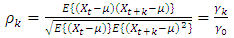 | (5) |
The autocovariance and autocorrelation are estimated by  where
where 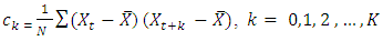 is the estimate of
  and
and  is the estimate of
  .
.
3.1.10. Diagnostic Checks
After fitting the model, the next step is to check whether the fitted model is adequate or not. This is accomplished by investigating the behaviour of the residuals. One of such ways is to examine the residual Autocorrelation function (ACF). If the ACF plot does not show any significant spike above or below the  line, then the model is adequate.This ACF test is equivalent to using Ljung-Box statistic which is defined as
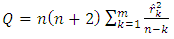 | (6) |
where n = the sample size and  is the estimated autocorrelation at lag k.In this test, the first m autocorrelations are examined for model adequacy. According to Box et al (2008), under the null hypothesis that the residual is random (i.e. the residuals are serially uncorrelated) against the alternative;
  . Thus, if the model is inappropriate, the average values of Q will be inflated. On the other hand if the model is adequate, the calculated Q will be less than
  obtained from the chi-square table. In other words, obtaining an adequate model means the residuals follow a white noise process.
3.2. Multivariate Time Series
The methods applied in the multivariate process are outlined below. The bold letters indicate vectors or matrices.
3.2.1. White Noise Process
A white noise process 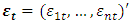 is a continuous random vector satisfying
  and
and  are independent for
  .
.
3.2.2. Cross Correlation
The cross correlation for  is given as
  | (7) |
 where
where  are the sample means of
  are the sample standard deviations respectively.
3.2.3. Vector Autoregressive (VAR) Model
The basic p-lag Vector autoregressive  model is of the form.
 | (8) |
where vector of time series variables,
 are fixed
  coefficient matrices,
 is a fixed
  vector of intercept terms allowing for the possibility of non zero mean
  ,
, is an
is an  vector white noise process or innovation process. That is,
 .
. Covariance matrix which is assumed to be non singular if not otherwise stated.The model can be written in the matrix form as
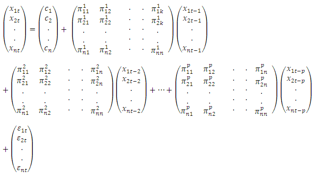 | (9) |
3.2.4. Stable VAR(p) Processes
The process (8) is stable if its reverse characteristic polynomial of the VAR(p) has no roots in and on the complex unit circle. Formally xt is stable if  | (10) |
A stable VAR(p) process  is stationary.
3.2.5. Autocovariances of a Stable VAR(p) Process
For a vector autoregressive process of order  we have
 | (11) |
Post multiplying both sides by  and taking expectation, we have for k = 0 using
 | (12) |
If 
 | (13) |
These equations can be used to compute the autocovariance functions  for
for  , if
, if  and
and 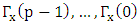 are known.
3.2.6. Autocorrelation of a Stable VAR(p) Process
For a stable VAR (p) process, the autocorrelations are given by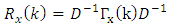 | (14) |
where D is a diagonal matrix with the standard deviation of the component of  on the main diagonal. Thus,
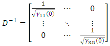 | (15) |
and the correlation between  and
and  is
is 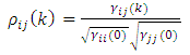 | (16) |
which is just the ij - th element of  .
.
3.2.7. VAR Order Selection
To determine the order of the VAR process, the three order selection criteria listed below are used:(i) Akaike Information CriterionThis is expressed as | (17) |
(ii) Hannan-Quin CriterionThis is given as  | (18) |
(iii) Schwarz CriterionThis can be expressed as | (19) |
For the three criteria, the order p is chosen so as to minimize the values of the criteria. In other words, we chose the lag p for which the values of the criteria are the smallest.where p is the VAR order, is the estimate of white noise covariance matrix
  ,n is the number of time series components of the vector time seriesN is the sample size.
3.3. Diagnostic Checks
The diagnostic checks of the fitted model involve examination of the behaviour of the residuals. The method to be used is the Lutkepohl (2005) approach. According to him; if  is the true correlation coefficients corresponding to the
  , then we have the following hypothesis test at 5% level to check whether or not a given multivariate series follows a white noise process or not. The hypothesis states:
 Against
 DecisionReject
  .Thus in practical sense, we compute the correlation of the series to be tested (possibly after some stationary transformation) and compare their absolute value with
  .
.
3.4. Model Evaluation
After fitting the univariate and the multivariate models and confirming the adequacy of the models; a comparative study between the two approaches shall be based on the following statistics:(i) The Mean Square Error (MSE)  (ii) The mean absolute error (MAE)
 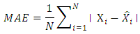 (iii) The mean absolute percentage error (MAPE)
 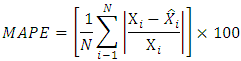 where
where  are the observed values (series) and
  are the estimated values.The performance evaluation is used to determine the model that is most efficient and reliable for modeling GDP variables.
4. Data Analysis and Results
The data used for this work is a quarterly data of the different sectors (variables) of the Nigerian Gross Domestic Products obtained from National Bureau of Statistics (NBS) for the period of 1981-2013. These different sectors are Agriculture  , Industry
  , Building & Construction
  , Wholesale & Retail
  and Services
  . The software used for the analysis are the gretl and Minitab.
4.1. Raw Data Plots
The raw data plots of the five series are displayed in figure 1 of the appendix A. From this plots, it is evidenced that the series are non-stationary; hence first differencing transformation was applied and stationarity was obtained. The differenced series are plotted in figure 2 of the appendix A.
4.2. Fitting the Univariate Models
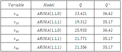
The different univariate models that were fitted to the different series  are displayed in table 1 below. The five models underwent diagnostic checks and were found to be adequate as informed by the values of Q statistics.
 Table 1. Fitted Univariate Models and the Computed Values of the Statistic
 |
| |
|
The first  autocorrelations were considered in the diagnostic checks. As highlighted in the methodology, the adequacies of the models are based on the fact that the
  are less than the
  .
.
4.3. Fitting the Multivariate Model
The autocorrelations of the five component series are displayed in table 2 below. The correlations are quite high indicating that the five variables are interrelated. Thus, multivariate technique can be applied. Table 2. Correlation Table of the Differenced Series
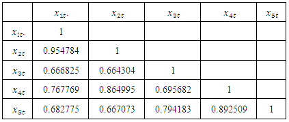 |
| |
|
4.4. Residual Cross Correlation
The residual cross correlations of the fitted univariate components are shown in table 3 below. As clearly seen, the cross correlations are quite high; suggesting strong relationship among the variables. Thus, multivariate consideration is obvious.Table 3. Residual Cross Correlation Table of the Differenced Series
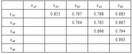 |
| |
|
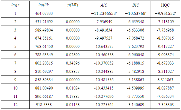
4.5. VAR Order Selection
Table 5 of the appendix A shows the values of the three model selection criteria at different lags. Clearly the three model selection criteria attain their minimum at lag 1 as indicated by the values with the asterisk. Thus, the selected model is VAR(1).
4.6. The Multivariate Model with the Significant Parameters
The multivariate VAR(1) time series model with the significant parameters is: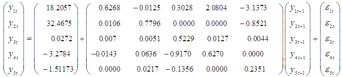 | (20) |
This can be expressed explicitely as: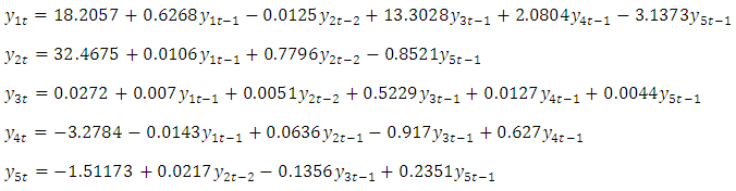
4.7. Stability of the VAR (1) Process
Using expression (10), the roots of  are
are 
 .Since
  , the process is stable. This also implies that the process is stationary.
5. Diagnostic Checks
The above fitted model (20) has to be subjected to diagnostics checks to ascertain whether the model is adequate or not. This is achieved by following the hypothesis stated in section 3.3 of the methodology. That is, Against
 Since
Since 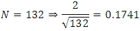 Then
Then is rejected if
 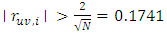 .Now, examining the residual correlation matrices at different lags in appendix B; it clearly shows that none of the residual autocorrelations
  is greater than 0.1741. In other words, the residuals follow a white noise process. This confirms the adequacy of the model.
6. Performances of the Estimated Models
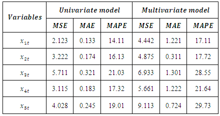
So far, adequate models have been fitted in the univariate and multivariate cases. The next step involves fishing out the most preferred models. This will be achieved by subjecting the models to the model evaluation test described in section 3.4 of the methodology. The test involves comparisons of the values of the different types of errors incurred by the models. The results are tabulated in table 4 below.Table 4. Error Comparison Table between Univariate and multivariate Models
 |
| |
|
As seen in the above table, the univariate models incur less error than the multivariate models in all the component series. Hence, the univariate model is the most efficient.
7. Discussion and Conclusions
Multivariate analysis has been embraced over the years; perhaps, due to its ability to carry other variables along. As noted in the review, Gabriel (2015) and others have celebrated multivariate methods and encouraged full attention towards it. The attention of many has been diverted from univariate modelling to multivariate analysis. However, the main goal of time series analysis is prediction, and a good model is the one that can predict the actual values of the data with less error. Of course, if a model can predict the real values of the data well; it is obvious that the forecasts are reliable. In this work, the truth is revealed. Despite the loud praises sung to multivariate models, its complications and newness, the univariate time series models with its simplicity have proven to perform better than the multivariate methods. It is therefore pertinent that model builders should not rely so much on the newness of any methods of analysis but should always carry out comparative analysis to determine the best option.
Appendix
Appendix A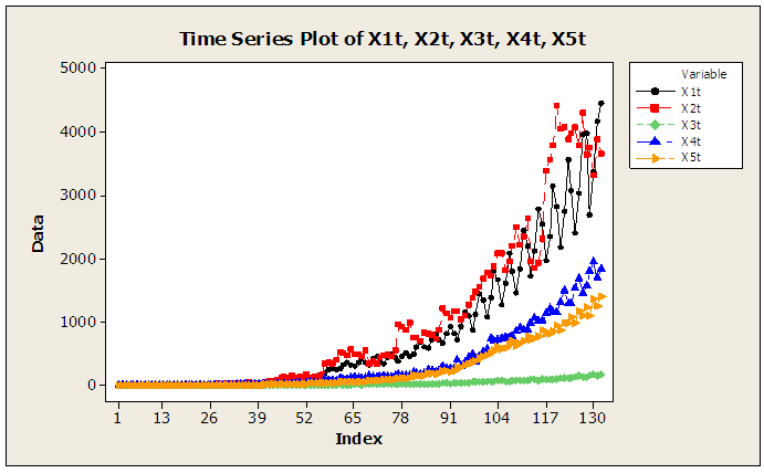 | Figure 1. Raw data plots of the series |
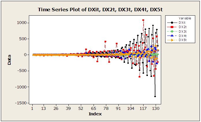 | Figure 2. Time series plots of the differenced series |
Table 5. Model selection criteria table
 |
| |
|
Appendix B: Residual Correlation Matrices (Ri Matrix for i = 0,1,2,…,10)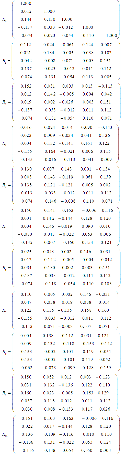
References
| [1] | Ben, K. A., Amos, H. J., Kenedy, W. and Bronze, T.S. (2010). Modelling non-linear multivariate data using non parametric methods. Journal of the American statistical association vol. 70, N0. 349 p.70-79. |
| [2] | Box, E.P., Jenkins, G.M. and Reinsel, G.C. (2008). Time Series Analysis, Forecasting and control. Wiley and Sons, Inc. Hoboken, New Jersey. ISBN: 978-0-470-27284-8(cloth). QA 280. B67 2008. 519.5’5 – dc22. |
| [3] | Elkhtem, S., G. and Karama, B. (2014); Multivariate function and tuning of crude distillation unit controller at Khartoum refinery – Sudan. Journal of applied and industrial Sciences, 2(3); 93-99. |
| [4] | Gabriel, P. K. (2015). On the application of Multivariate Times Series Models. Journal of Physical Science and Technology. Vol. 8; No. 10; pp 51-62. ISBN: 3-4428-321-9. |
| [5] | George, J. M. (2005). Comparative study of ARMA and Transfer function models. Ekonomicke rozhiady, vol. 30 No.4, p.457-466. |
| [6] | Henry, E. H. and Prebo, S. (2005). Analysis of time dependent geophysical variables. Journal of quality technology, vol.31, No. 3. pp. 34-41. ISBN: 4-312-50142-4. |
| [7] | Makridakis, H. and Clay, F.M. (2012). Forecasting: Methods and Applications, 3rd Ed. New York: John Wiley and Sons, pp. 373, 520-542, 553-574. ISBN: 925-0-520-22181-8. |
| [8] | Oluwatomi L, Bruce T. and Owa, H. (2011). Multivariate function for the study of Brazilian inflationary process. African Journal of Business Management. Vol 5(4): pp.468-482. |
| [9] | Saul, J., Parscal, D., Berger, W; Rao C., and Richard, J. (2013); Mulivariate analysis of autonomic regulation II. Respiratory sinus arrhythmia. Physiol. 256(heart circ.physiol. 25); H153-H161. |

 Abstract
 Reference
 Full-Text PDF
 Full-text HTML