Ehab A. M. Frah1, 2
1Department of Statistics, Faculty of Sciences, University of Tabuk, KSA
2Department of Statistics, Social and Economic Studies, University of Bahri, Sudan
Correspondence to: Ehab A. M. Frah, Department of Statistics, Faculty of Sciences, University of Tabuk, KSA.
| Email: |  |
Copyright © 2016 Scientific & Academic Publishing. All Rights Reserved.
This work is licensed under the Creative Commons Attribution International License (CC BY).
http://creativecommons.org/licenses/by/4.0/

Abstract
Sorghum is the largest crop in Sudan, where Sudan is one of the most important countries producing sorghum in the world. Sudan is the fifth country after China, India, USA and Nigeria in sorghum production worldwide. Sorghum is the most important crop and livestock feed. The study aims at forecasting the sorghum production in Sudan. The study using Box-Jenkins methodology in time series analysis which is the optimal method applied to the pattern. This method consists of four steps namely identification, estimation, diagnostic checking, and forecasting by ARIMA models. Future forecasts drawn there show that the sorghum production will be likely to increases in coming years.
Keywords:
ARIMA, Forecasting, Sorghum and Sudan
Cite this paper: Ehab A. M. Frah, Sudan Production of Sorghum; Forecasting 2016-2030 Using Autoregressive Integrated Moving Average ARIMA Model, American Journal of Mathematics and Statistics, Vol. 6 No. 4, 2016, pp. 175-181. doi: 10.5923/j.ajms.20160604.06.
1. Introduction
Sorghum is the fifth most important cereal crop grown in the world and is used for food, fodder and production of alcoholic beverages. Overall it is an important crop type of food in Africa, Central America and South Asia. Food and Agriculture Organization (FAO) reported. The average annual yield in 2010 across the world was reported as 1.37 Tone’s/Ha, with the highest yields recorded in Jordan (12.7 T/Ha). In the USA this figure was 4.5 T/Ha. Sorghum is the staple food for most people living in Sudan, except for the northern areas (Nahr al-Nil and Northern states) where wheat is more common. Sorghum is the largest crop (ranked by area) in Sudan with about 6.5 million Ha grown in 2009 [1].Most of it is rain-fed. The geographical of distribution of sorghum is; Gadarif State (eastern Sudan) is the most important region for sorghum production, where about 5-6 million feddan are cultivated on an annual basis. Mainly to large scale farming where agricultural machinery is used. The dominant varieties grown are the traditional (Feterita) types e.g. (Arfa Gadmek, Abdalla Mustafa, Korolo. Tetron and Dabar) are grown on a limited scale. Some progressive farmers in south Gadarif grow the improved varieties, Wad Ahmed and Tabat. Sudan was exporting some quantities of sorghum in the 80’s and 90’s but reached almost zero levels in 2000. At the same time Sudan started to import 300 to 400 thousand Tonnes per year to cover its needs. Sorghum cannot be planted until soil temperatures have reached 17°C and requires an average temperature of at least 25°C to produce maximum grain yields while maximum photosynthesis potential is achieved at daytime temperatures of around 30°C. Night time temperatures below 13°C for more than a few days can severely affect potential grain production. Sorghum is drought tolerant and is able to grow economically in low rainfall areas, below 450 mm. However, in order to achieve high yields 100mm rainfall equivalent irrigation water should be applied per month if sufficient rainfall does not occur. Soil should be subject to soil analysis for nutrients availability. Organic manure and nitrogen fertilizers are the two main sources of plant nutrition when sufficient water is available through rainfall or irrigation. Most of the crop is manually harvested and left in open air to dry until grain moisture content is below 10%. Usually sowing takes place from mid-June until mid-July. Timing is very important for achieving yield potential as the growing season is long (usually 90–120 days) and late sown crops suffer loss of production. Seed rate is typically 3 Kg/Feddan which is enough to produce 42000–52000 plants per Feddan. In rain-fed areas this rate can be increased to 3.5Kg per Feddan to compensate for the less favorable conditions [2].Africa accounts only for a quarter of world's sorghum production. Nigeria and Sudan contribute nearly half of the sorghum production in Africa [3]. Sudan is one of the most important countries producing sorghum in the world. It has the fifth rank after China, India, USA and Nigeria in sorghum production, but it is number one in per capita area and grain consumption for human beings [4].Sudan shares in total sorghum production which is amounting to 6.51% and 19.6% of the world and Africa production respectively in 2009/2010 season. Sorghum is produced in the three sub-sectors in the Sudan, namely; the irrigated, mechanized and traditional rainfed subsectors. The traditional rainfed sub-sector is mainly found in Kordofan, Darfur plus a large area in the Central States. The contribution of this sub-sector to the total sorghum output is estimated at only 29.91 percent (about 541 thousand metric tons) from an area of about 1.353million feddan in 2011/12. The low share of this sub-sector is due to the production of sorghum mainly for subsistence [4].
2. Sorghum Production Model
As is generally known, developing a time series model from such data starts by exploring the main features inherent in the series. Among these features are stationarity and the existence of seasonality (cyclical pattern) in the data. Appropriate statistical procedures will now be used for investigating these aspects of the series in an attempt to determine the suitable time series model that fits it.
2.1. Testing for Stationarity
Stationary series vary around the constant mean level, neither decreasing nor increasing systematically over time, with constant variance. Certain time series models, namely Box-Jenkins model, assume the existence of stationarity. General Box-Jenkins model includes difference operators, autoregressive terms, moving average terms, seasonal difference operators, seasonal autoregressive terms, and seasonal moving average terms. This phase is founded on the study of autocorrelation and partial autocorrelation. The Box-Jenkins model assumes the stationarity of the series under investigation, which means that the series has constant mean, constant variance, and constant autocorrelation structure. Thus first step in developing a Box-Jenkins model is to determine if the series is stationary and if there is any significant seasonality that needs to be modeled [5].Consider the AR (1) model: | (1) |
For this model the autoregressive polynomial equation is  and therefore is the root of the autoregressive polynomial. Thus, for the AR (1) model to be stationarity it is required that
  and therefore
  Similarly, for an MA (1) model
  to be invertible it is required that
  and therefore
  For the stationarity and invariability conditions for other popular Box-Jenkins models like the AR (2), MA (2), and ARMA (1,1) models, see ADF and PACF result. By definition, all AR (p) models are invertible while all MA (q) models are stationarity.
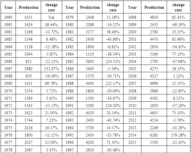
Table (1). Sudan Sorghum production annually 1960-2015
 |
| |
|
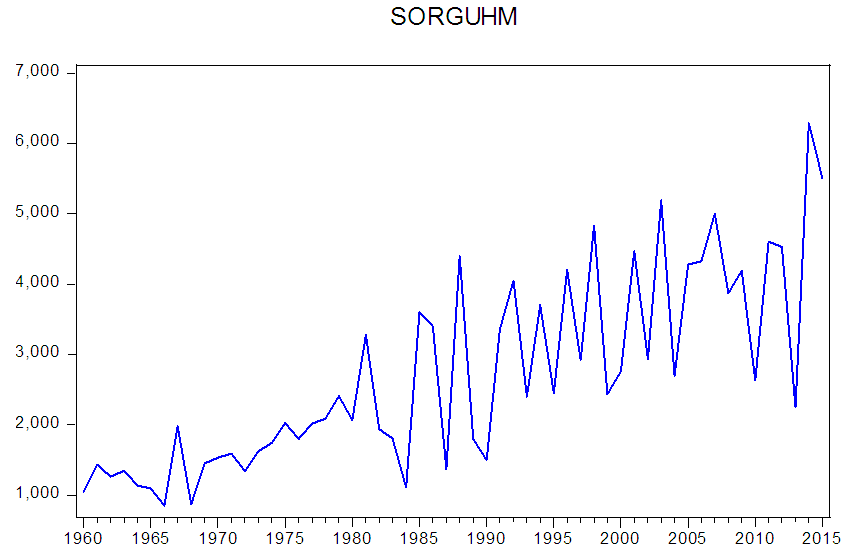 | Figure (1). Show the Sudan sorghum production 1960-2015 |
Now consider the practical implications of stationarity and invariability in Box-Jenkins models. When a Box-Jenkins model is stationarity, its observations yt satisfy the following three properties: 1.  (i.e. the mean of
  is constant for all time periods) 2.
  (i.e. the variance of
  is constant for all time periods) 3.
 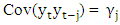 (i.e. the covariance between
  is constant for all time periods and fixed j, j = 1, 2,) These three conditions give rise to what is called weak stationarity (or just stationarity for short). The practical implication of stationarity is that only one realization of the time series yt is needed for us to be able to consistently estimate the mean μ, the variance
  the covariance
  and the autocorrelation
  with the sample statistics
  and
and  These statistics are defined as:
 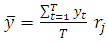 | (2) |
where T denotes the total number of observations available on yt (sample mean)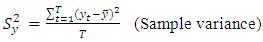 | (3) |
 | (4) |
 | (5) |
Stationarity can be accessed from a run sequence plot. The run sequence plot should show constant location and scale. It can also be detected from an autocorrelation plot. Specifically, non-stationarity is often indicated by an autocorrelation plot with very slow decay.Box and Jenkins recommend differencing non-stationary series one or more times to achieve stationarity. Doing so produces an ARIMA model, with "I" short for "Integrated". But its first difference, expressed as  is stationary, so y is integrated of order 1”, or
2.2. Seasonality in Box-Jenkins Models
Box-Jenkins models can be extended to include seasonal autoregressive and seasonal moving average terms. Model identification: seasonality of order s is revealed by "spikes” at s, 2s, 3s, lags of the autocorrelation function. Model estimation: to make a series stationary, may need to take sth differences of the raw data before estimation. These seasonal effects may themselves follow AR and MA processes. At the model identification stage, our goal is to detect seasonality, if it exists, and to identify the order for the seasonal autoregressive and seasonal moving average terms. For Box-Jenkins models, it isn’t necessary to remove seasonality before fitting the model. Instead, it can include the order of the seasonal terms in the model specification to the ARIMA estimation software. Once stationarity and seasonality have been addressed, the next step is to identify the order (the p and q) of the autoregressive and moving average terms. The primary tools for doing this are the autocorrelation plot and the partial autocorrelation plot. The sample autocorrelation plot and the sample partial autocorrelation plot are compared to the theoretical behaviour of these plots when the order is known.
2.3. Order of Autoregressive Process (p)
Specifically, for an AR(1) process, the sample autocorrelation function should have an exponentially decreasing appearance. However, higher-order AR processes are often a mixture of exponentially decreasing and damped sinusoidal components. For higher-order autoregressive processes, the sample autocorrelation needs to be supplemented with a partial autocorrelation plot. The partial autocorrelation of an AR (p) process becomes zero at lag p+1 and greater, so we examine the sample partial autocorrelation function to see if there is evidence of a departure from zero. This is usually determined by placing a 95% confidence interval on the sample partial autocorrelation plot (most software programs that generate sample autocorrelation plots will also plot this confidence interval). If the software program does not generate the confidence band, it is approximately ±2/N, with N denoting the sample size. The data is AR (p) if: ACF will decline steadily, or follow a damped cycle and PACF will cut off suddenly after p lags.
2.4. Order of Moving Average Process (q)
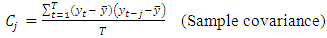
The autocorrelation function of a MA (q) process becomes zero at lag q+1 and greater, so we examine the sample autocorrelation function to see where it essentially becomes zero. Alternating positive and negative, Autoregressive model. Use the partial autocorrelation plot to decaying to zero help identify the order. One or more spikes, rest are Moving average model, order identified by where plot essentially zero becomes zero. Decay, starting after a few lags mixed autoregressive and moving average model. All zero or close to zero Data is essentially random. High values at fixed intervals Include seasonal autoregressive term. No decay to zero series is not stationary.The data is MA (q) if: ACF will cut off suddenly after q lags and PACF will decline steadily, or follow a damped cycle. It’s not indicated to build models with: – Large numbers of MA terms – Large numbers of AR and MA terms together, well see very (suspiciously) high t-statistics.This happens because of high correlation (“collinearity”) among regressors, not because the model is good. It is observable from Fig (2) above that the time series is likely to have random walk pattern. More over ACFs suffered from linear decline and there is only one significant spike for PACFs. The correlogram also suggests that ARIMA (1, 0, 0) may be an appropriate model. Then, we take the first-difference of "sorghum” to see whether the time series becomes stationary before further finding AR (p) and MA (q). | Figure (2). First difference Sudan sorghum production (1960-2015) |
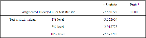
To realise whether first difference can get level-stationary time series or not, so the results are: Now, the first-difference series "sorghum" becomes stationary as shown in line graph Figure (3) and is white noise as it shows no significant patterns in the graph of correlogram Figure (4). And the unit root test also confirms the first-difference becomes stationary since the ADF value is less than 1% Critical Value l.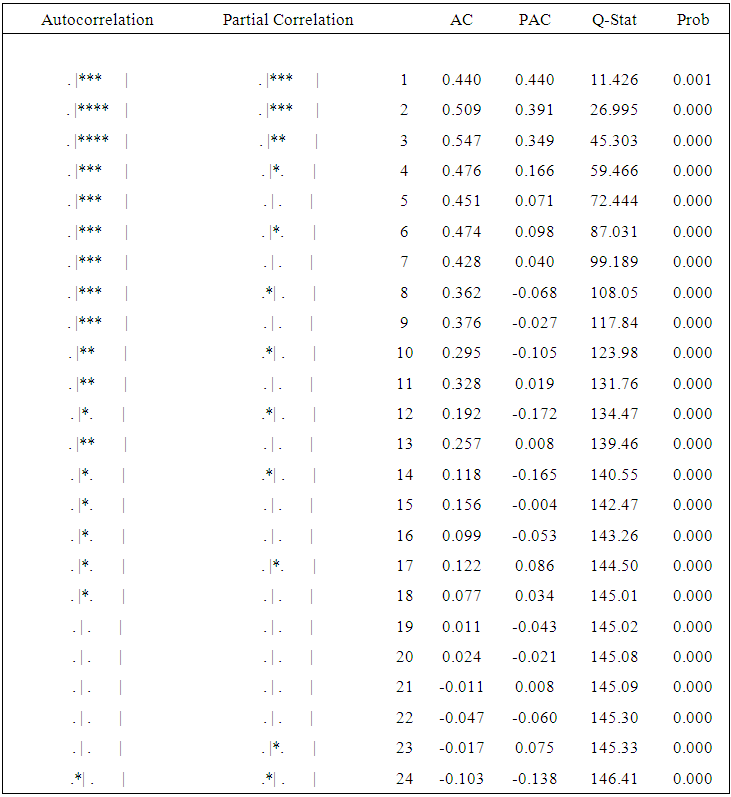 | Figure (3). Correlogram graph Sudan sorghum production (1960-2015) |
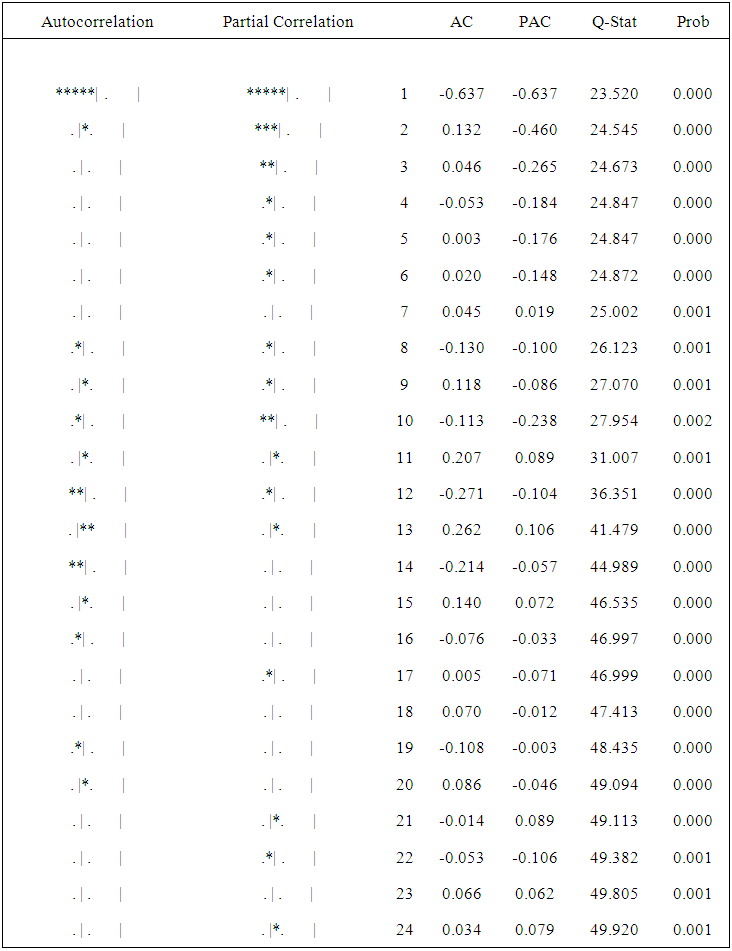 | Figure (4). Correlogram graph of the first difference Sudan sorghum production (1960-2015) |
2.5. Box-Jenkins Model Estimation
The main approaches to fitting Box-Jenkins models are non-linear least squares and maximum likelihood estimation. Maximum likelihood estimation is generally the preferred technique. (Box & Jenkins; 1994).
3. Box-Jenkins Model Diagnostics
Model diagnostics for Box-Jenkins models is similar to model validation for non-linear least squares fitting. That is, the error term ut is assumed to follow the assumptions for a stationary unvaried process. The residuals should be white noise (or independent when their distributions are normal) drawings from a fixed distribution with a constant mean and variance. If the Box-Jenkins model is a good model for the data, the residuals should satisfy these assumptions. If these assumptions are not satisfied, we need to fit a more appropriate model. That is, we go back to the model identification step and try to develop a better model.Hopefully the analysis of the residuals can provide some clues as to a more appropriate model. The residual analysis is based on: 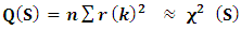 | (6) |
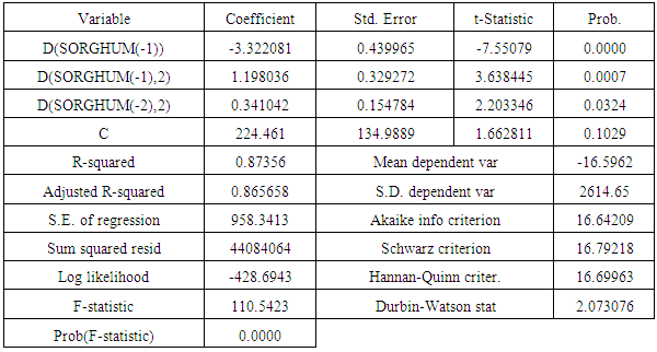
1. Random residuals: the Box-Pierce Q-statistic: where r(k) is the k-th residual autocorrelation and summation is over first s autocorrelations. 2. Fit versus parsimony: the Schwartz Bayesian Criterion (SBC): SBC = ln {RSS/n} + (p+d+q) ln (n)/n, where RSS = residual sum of squares, n is sample size, and (p+d+q) the number of parameters. Having investigation the main feature of sorghum production data for 1960 – 2015 in an attempt the lay the foundation for choice of the appropriate method of fitting a model which best fits the data, and having conclude that the as in table one is an RIMA (1, 1) model it is now time for fitting it to the data .i.e its parameters be will now obtained from sorghum production data.Model with high adjusted R2 indicates that the regression line perfectly fits the data, small value of Akaike info criterion is best model and Durbin-Watson around 2 indicates no autocorrelation in the model Table (3).Table (2). Dukey f test first difference of Sudan sorghum production (1960-2015)
 |
| |
|
Table (3). Model parameter
 |
| |
|
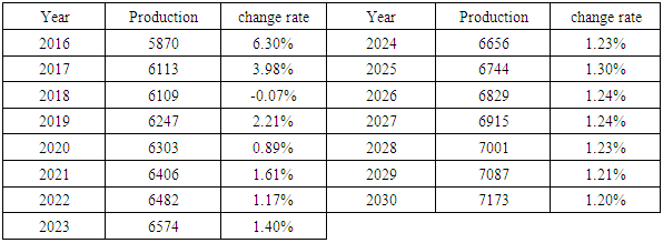
Table (4). Show Sorghum production forecasting
 |
| |
|
The findings have shown that between 1960 and 2015, Sudanese sorghum production at an annual increasing. Growth in production is attributed to changes in harvested area land. To more increase productivity growth, farmers should be provided with new technology, access to modern inputs, and adequate logistical support.
4. Conclusions
The forecasting findings have shown that between 1960 and 2015, Sudanese sorghum production at an annual increasing. Growth in production is attributed to changes in harvested area land. For more increase productivity growth, farmers should be provided with new technology, access to modern inputs, and sufficient logistical support.
References
| [1] | Food and Agriculture Organization (FAO) (1997). FAO/WFP Crop and Food Supply Assessment Mission to Sudan. Special Report. Rome. |
| [2] | Food and Agriculture Organization (FAO) and International Crop Research Institute for the Semi-Arid Tropics (ICRISAT) (1996). The World Sorghum and Millet Economies Facts, Trends and Outlook. FAO and ICRISAT. Rome. |
| [3] | Robert M. Ogeto, Erick Cheruiyot, Patience Mshenga and Charles N. Onyari (2013). Sorghum production for food security: A socioeconomic analysis of sorghum production in Nakuru County, Kenya. |
| [4] | Hassan, Thabit Ahmed (2002) Instability of the main Food Grain (Millet and Sorghum) Production in the Sudan with Reference to South Darfur State, unpublished PhD Faculty of Agriculture, U of K. |
| [5] | Box GEP, Jenkins GM (1970). Time Series Analysis, Forecasting and Control. Holden Day, San Francisco. pp.46-87. |

 Abstract
 Reference
 Full-Text PDF
 Full-text HTML