Alkreemawi Walaa Khazal1, 2, Wang Xiang Jun1
1School of Mathematics and Statistics, Huazhong University of Science and Technology, Wuhan, China
2Department of Mathematics, College of Science, Basra University, Basra, Iraq
Correspondence to: Alkreemawi Walaa Khazal, School of Mathematics and Statistics, Huazhong University of Science and Technology, Wuhan, China.
| Email: |  |
Copyright © 2016 Scientific & Academic Publishing. All Rights Reserved.
This work is licensed under the Creative Commons Attribution International License (CC BY).
http://creativecommons.org/licenses/by/4.0/

Abstract
A stochastic differential equation (SDE) defines N independent stochastic processes The drift term depends on the random variable
  . The distribution of the random effect
  depends on unknown parameters, which are to be estimated from continuous observation of the processes
  . When the drift term is defined linearly on the random effect
  (additive random effect) and
  has a Gaussian mixture distribution, we obtain an expression of the exact likelihood. When the number of components is known, we prove the consistency of the maximum likelihood estimators
  . The convergence of the EM algorithm described when the algorithm is used to compute
  .
.
Keywords:
Maximum likelihood estimator, Mixed effects stochastic differential equations, Consistency, EM algorithm, Mixture distribution
Cite this paper: Alkreemawi Walaa Khazal, Wang Xiang Jun, Consistency of Estimators in Mixtures of Stochastic Differential Equations with Additive Random Effects, American Journal of Mathematics and Statistics, Vol. 6 No. 4, 2016, pp. 162-169. doi: 10.5923/j.ajms.20160604.04.
1. Introduction
A mixture model (MM) is beneficial for modeling data as output from one of several groups, clusters, or classes; the groups (clusters, classes) might be different from each other, but the observations within the same group are similar to each other. In this paper, we concentrate on the classification problem of longitudinal data modeled by a stochastic differential equation (SDE) with random effects that have a mixture of Gaussian distributions. Some researchers state that the classes are known, whereas other researchers state the opposite. Arribas-Gil et al. [1] and references therein assumed that the classes are known and deal with classification drawbacks of longitudinal data by using random effects models or mixed-effects models. Their aim is to establish a classification rule of longitudinal profiles (curves) into a number that enables dissimilar classes to predict the class of a new individual. Celeux et al. [6] and Delattre et al. [9] assumed that the numbers of classes are unknown. Celeux et al. [6] used maximum likelihood with the EM algorithm to estimate the random effects within a mixture of linear regression models that include random effects (see, Dempster, A. et. al. [10]), and they used Bayesian information criterion (BIC) to select the number of components. Delattreet al. [9] used maximum likelihood to estimate the random effects in SDE with multiplicative random effect in the drift and diffusion terms without random effects with the EM algorithm (Dempster, A. et. al. [10]). They also used BIC to select the number of components. Delattre et al. [9] studied SDEs with the following form: | (1) |
where  are
are  independent Wiener processes,
  are
are  independently and identically distributed
  random variables. The processes
  are also independent on random variables
  , and
, and  is a known real value. The drift function
  is a known function defined on
  and the functions
  . Each process
  represents an individual, and the random variable
  represents the random effect of individual i.Delattre et al. [2] considered the special case (multiple case) where
  is linear in
  ; in other words,
  , where
  is a known real function, and
  has a Gaussian mixture distribution.Here, we consider functional data modeled by a SDE with drift term
  depending on random effects where
  is linear in random effects
  (addition case),
  and diffusion term without random effects. We consider continuous observations
  with a given
  . Here,
  are unknown parameters in the distribution of
  from the
  which will be estimated, but the estimation is not straightforward. Generally, the exact likelihood is not explicit. Maximum likelihood estimation in SDE with random effects has been studied in a few papers (Ditlevsen and De Gaetano, 2005 [11]; Donnet and Samson, 2008 [12]; Delattre et al. (2013) [8]; Alkreemawi et al. ([2], [3]); Alsukaini et al. ([4], [5]). In this paper, we assume that the random variables
  have a common distribution with density
  for all
  , which is given by a mixture of Gaussian distributions; this mixture distribution models the classes. We aim to estimate unknown parameters and study the proportions.
  is a density with respect to a dominant measure on
  , where
  is the real line, and
  is the dimension.
 with
with  as the proportions of the mixture
  ,
,  as the number of components in the mixture, and
  and
and  a
a  as an invertible covariance matrix. Let
  denote the true value of the parameter. M is the number of components and is known.
  is set for the unknown parameters to be estimated. Our aim is to find estimators of the parameters
  of the density of the random effects from the observations
  . We focus on an additional case of linear random effects
  in the drift term
  . In addition, we prove and explain that the observations concerning exact likelihood are explicit. With M as the number of known components, we discuss the convergence of the EM algorithm, and the consistency of the exact maximum likelihood estimator is proven. The rest of this paper is organized as follows: Section 2 contains the notation and assumptions, and we present the formula of the exact likelihood. In Section 3, we describe the EM algorithm and discuss its convergence. In Section 4, the consistency of the exact maximum likelihood estimator is proved when the number of components is known.
2. Notations and Assumptions
Consider the stochastic processes  , which are defined by (1). The processes
  and the random variables
  are defined on the probability space
  . We use the assumptions (H1, H2, and H3) in Delattre et al. [9]. Consider the filtration
  defined by
  .H1. The functions
  and
and  are Lipschitz continuous on
  and
and  is Hölder continuous with exponent
  on
on  .By (H1), for
  , for all
  , the stochastic differential equation
  | (2) |
admits a unique solution process  adapted to the filtration
  , Moreover, the stochastic differential equation (1) admits a unique strong solution adapted to
  such that the joint process
  is strong Markov and the conditional distribution of
  given
given  is identical to the distribution of (2). (1) shows that the Markov property of
  is straightforward as the two-dimensional SDE
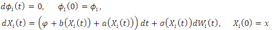 The processes
  are
are  (see Delattre et al. [8]; Genon-Catalot and Larédo [13], Alkreemawi et al. [2], [3]; Alsukaini et al. [4], [5]). To derive the likelihood function of our observations, under (H1), we introduce the distribution
  on
on  given by (2), where
  denotes the space of real continuous functions
  defined on
  endowed with the
  associated with the topology of uniform convergence on
  . On
. On  , let
, let 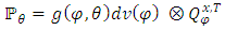 denote the joint distribution of
  , and let
  denote the marginal distribution of
  on
on  . Also, we denote
  ,
,  (resp.
  ) the distribution
  of
of  where
where  has a distribution
  (resp. of
  ), with these notations
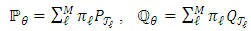 | (3) |
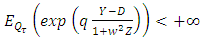
H2. For all  ,
, We denote by
  , with
 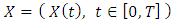 , which is the canonical process of
  . Under (H1)–(H2), based on Theorem 7.19 p. 294 in [14], the distributions
  and
and  are equivalent. Through an analog approach of [9], the following results are used:
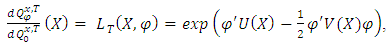 where
where  is the vector, and
  is the
  matrix
 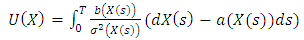 | (4) |
and  is the
  matrix
 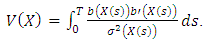 | (5) |
Thus, the density of  (the distribution of
  on
on  ) with respect to
  is obtained as follows:
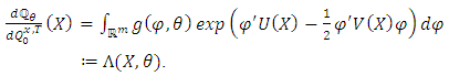 | (6) |
The exact likelihood of  is
is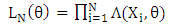 | (7) |
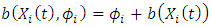
Thus, for our situation (addition situation) of drift where is linear in
  ,
, 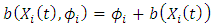 , we have
 and,
and,  | (8) |
where 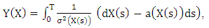 | (9) |
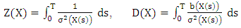 | (10) |
We have to consider distributions for  such that the integral (8) can obtain a tractable formula for the exact likelihood. This is the case when
  has a Gaussian distribution and the drift term
  is linear in
 ,
,  (addition situation), as shown in Alkreemawi et al. [2]. This is also the case for the larger class of Gaussian mixtures. The required assumption is defined as follows:H3. The matrix
  is positive definite
  and
and  for all
  .(H3) is not true when the functions
  and
and  are not linearly independent. Thus, (H3) can ensure a well-defined dimension of the vector
  .Proposition 2.1. Assume that
  is a Gaussian mixture distribution, and set
 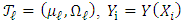 ,
, ,
,  ,
,  ,
,  . Under (H3), the matrices
  are invertible
  and
and  for all
  . By setting
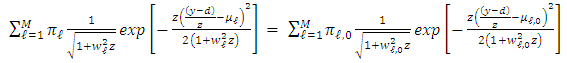
 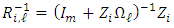 , we obtain,
 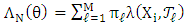 | (11) |
where 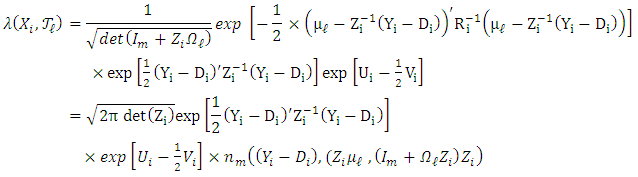 | (12) |
Here, 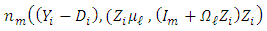 denotes the Gaussian density with mean
  and covariance matrix
  .Alkreemawi et al. [2] considered the formula for
  (Proposition 3.1.1 and Lemma 4.2). The exact likelihood (7) is explicit. Hence, we can study the asymptotic properties of the exact MLE, which can be computed by using the EM algorithm instead of maximizing the likelihood.
3. Estimation Algorithm
In the situation of mixtures distributions with number of components M, M is known, rather than of solving the likelihood equation, we use the EM algorithm to find a stationary point of the log-likelihood. A Gaussian mixture model (GMM) is helpful for modeling  by using a mixture of distributions, which means that the population of individuals is grouped in M clusters. Formally, for the individual i, we (may) introduce a random variable
  , with
  and
and 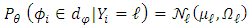 . We assume that
  are
are  and
and  independent of
  . The concept of the EM algorithm was presented in Dempster et al. [10] which considered the data
  as incomplete and introduced the unobserved variables
  . Simply, in the algorithm, we can consider random variables
  where
where  , for
, for  ; such values indicate that the density component drives the equation of subject i. For the complete data
  , the logarithm likelihood function is explicitly given by
  | (13) |
The EM algorithm is an iterative method in which the iteration alternates between performing an expectation (E) step, which is the computation of where
where  is the conditional expectation given
  computed with the distribution of the complete data under the value
  of the parameter, and the maximization (M) step computes parameters that maximize the expected log-likelihood found on the (E) step
  . In the (E) step, we compute
 where
where  is the posterior probability
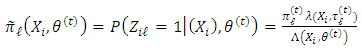 | (14) |
In the EM algorithm, at iteration n, we want to maximize  with respect to
  , where
  is the current value of parameter
  . We can maximize the terms that contain
  and
and  separately. We introduce one Lagrange multiplier
  to maximize with respect to
  with the constraint
  and solve the following equation:
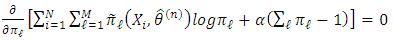 And the classical solution:
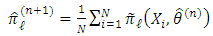 Then, we maximize
 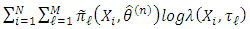 , where the derivatives can be computed with respect to the components of
  and
and  by using some results from matrix algebra. When taking the log of
  , substituting it into
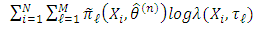 , and taking the derivative w.r.t.
  , we have
 | (15) |
When the  are known and when the
  are unknown, the maximum likelihood estimators of the parameters are given by the system.Proposition 3.1 The sequence
  generated by the EM algorithm converges to a stationary point of the likelihood.Proof. We prove the convergence for
  to avoid cumbersome details. We employ the results obtained by McLachlan and Krishnan [15]. As the following conditions are given:
 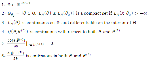 Conditions 3, 4, 5, and 6 are verified by the regularity of the likelihood (see Proposition 4.2). In a standard Gaussian mixture, condition 2 is usually unverified (see McLachlan and Krishnan [15]. However, here, one has the following result (see (12)):
 Where
Where  . Therefore, the formula of
  is a mixture of Gaussian distributions that consist of variances all bounded from below. This finding reveals condition 2.
4. Asymptotic Properties of MLE
This section aims to investigate theoretically the consistency and asymptotic normality of the exact maximum likelihood estimator of  when we assume that the number of components M is known. For simplicity’s sake, we consider only the case
  . The parameter set
  is given by
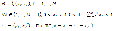 Now, we set
 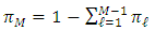 , but only
  parameters need to be estimated. When necessary in notations, we set
  . The MLE is defined as any solution of
 where
where  is defined by (7)–(11). To prove the identifiability property, the following assumption is required as in Alkreemawi et al. [2]:(H4) Either the function
  is constant or not constant, and under
  , the random variable
  admits a density
  with respect to the Lebesgue measure on
  , which is jointly continuous and positive on an open ball of
  .When
.When  is constant, this case is simple. For instance, let
  . Then,
  is deterministic, and under
  . Under
 is a mixture of Gaussian distributions with means
  , variances
  , and proportions
  .The case where
  is not constant. Under smoothness assumptions on functions
  , assumption (H4) will be accomplished by using Malliavin calculus tools (see Alkreemawi et al. [2]). As mixture distributions are utilized, the identifiability of the entire parameter
  can only be obtained in the following concept:
 | (16) |
Now, we can prove the following:Proposition 4.1. Under (H1)-(H2)-(H4),  implies that
  .Proof. First, when
  is not constant, we consider two parameters
  and
and  , and aim to prove that
  implies
  . As
. As  and
and  depend on
  only through the statistics
 with a slight abuse of notation, we set
  and
and | (17) |
Under (H4),  is the density of the distribution of
  under
under  with respect to the density of
  under
under  and
and  implies
  a.e., hence, everywhere on
  by the continuity assumption. We deduce that the following equality holds for all
 Let us set
 and
and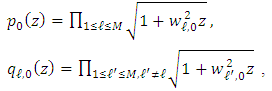 We note that
  . Thus, such quantities do not depend on
  . After reducing to the same denominator, we obtain
 The right-hand side is a function of
  , whereas the left-hand side is a function of z only. This approach is possible only if
  for all
  . Therefore,
  | (18) |
and the equality of the variances can be obtained by reordering the terms if required. Then, we have for  and a fixed z,
 | (19) |
Here,  indicates the Gaussian density with mean m and variance
  . Analogously, by using the equality (18),
 For all fixed
  , we therefore have for all
  ,
,  Herein, the equality of two mixtures of Gaussian distributions with proportions
  , expectations
  and
and  , and the same set of known variances
  are given. From the identifiability of Gaussian mixtures, we have the equality
 and thus,
  .Second, when
  is constant, for instance, let
  . As noted above, under
  and
and  . Therefore,
  is a Gaussian distribution. Under
  ,
,  has density
  w. r. t. the Lebesgue measure on
  . Specifically, the mixture of Gaussian densities can also be deduced based on the identifiability property of Gaussian mixtures.Proposition 4.2. Let
  denote the expectation under
  . The function
  is
is  on
on  and
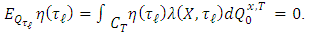
and 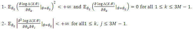
 for all
  .The Fisher information matrix can be defined as
 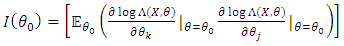 for all
  . Proof. We use results proved in Alkreemawi el al. [2] (Section 3.1, Lemma 3.1.1, Proposition 3.1.2) to prove this proposition. For all
  and all
  ,
,
 is the distribution of
  when
when  has a Gaussian distribution with parameters
  . This idea implies that
 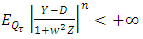 for all
  . Let
. Let The random variable that has moments of any order under
  is bounded, and the following relations hold:
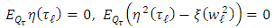 | (20) |
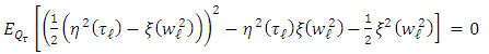 | (21) |
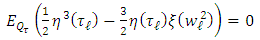 | (22) |
All derivatives of  are well defined. For
  , we have
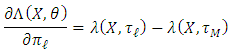 As for all
 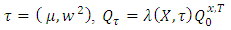 , the random variable above is
  -integrable and
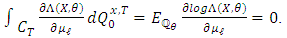
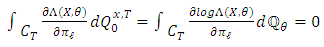 Moreover, as
 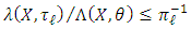 , we have
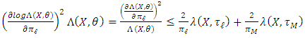 Therefore,
 Higher order derivatives of
  with respect to the
  are nul:
 Now we find the derivatives with respect to the parameters
  . We have:
  We know that:
 Consequently,
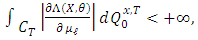
 Now,
Now,  Thus,
Thus,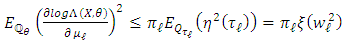 Next, we have
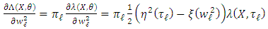 Again, we know that this random variable is
  -integrable with nul integral, thereby obtaining
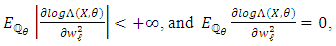 Moreover,
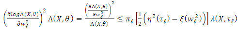 This finding implies that
 Now we look at second-order derivatives. The successive derivatives with respect to
  with
with  are nul. We obtain
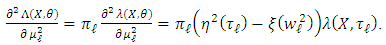 This random variable is integrable with respect to
  with the nul integral. Thus,
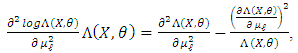 We find that this random variable is integrable with respect to
  , and computing the integral obtains
 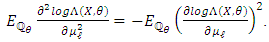 Next,
Next,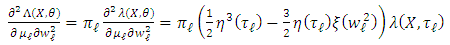
 Thus, we conclude the proof analogously using (21) and (22).Proposition 4.3. Assume that
  is invertible and (H1)–(H2). Then, an estimator
  solves the likelihood estimating equation
  with a probability tending to 1 and
  in probability.Proof. For weak consistency following the standard steps, the uniformity condition needs to be proven. We prove that An open convex subset
  of
of  exists, which contains
  and functions
  such that, on S,
 .
. are set as positive numbers such that
  , and
, and  is assumed to belong to
  where
where  . We have to study
 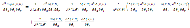 Therefore, we have, for
  distinct indexes
 As
As  ,
, We use
  again to bound the other third-order derivatives. Then, in the derivatives, random variables appear
 for different values of n. We now bound
  by an r. v. independent of
  and have moments of any order under
  . We have
 Thus,
Thus, Now, in the same method
  For all
  , this finding implies that
 Consequently,
 The proof of Proposition 4.3 is complete.
5. Conclusions
In stochastic differential equations based random effects model framework. We considered the addition case in the drift where  is linear in
  , where
  has a mixture of Gaussian. We obtain an expression of the exact likelihood. When the number of components is known, we prove the consistency of the maximum likelihood estimators (MLEs). Properties of the EM algorithm are described when the algorithm is used to compute MLE.
ACKNOWLEDGEMENTS
The Author is grateful to Dr. Wang Xiang jun of School of Mathematics and Statistics, Huazhong University of Science and Technology, Wuhan, Hubei, 430074 P.R. China. Also, to Mr. Alsukaini M. S. of the department of Mathematics, College of Science, Basra University, Basra, Iraq for their constructive comments.
References
| [1] | Arribas-Gil, A., De la Cruz, R., Lebarbier, E. and Meza, C. (2015). Classification of longitudinal data through a semiparametric mixed-effects model based on lasso-type estimators. Biometrics 71, 333–343. |
| [2] | Alkreemawi W. K., Alsukaini M. S. and Wang X. J. “On Parameters Estimation in Stochastic Differential Equations with Additive Random Effects,” Journal of Advances in Mathematics, Vol. 11, no.3, 5018 – 5028, 2015. |
| [3] | Alkreemawi W. K., Alsukaini M. S. and Wang X. J. “Asymptotic Properties of MLE in Stochastic Differential Equations with Random Effects in the Drift Coefficient,” International Journal of Engineering, Science and Mathematics (IJESM), Vol. 5, Issue. 1, 1 – 14, 2016. |
| [4] | Alsukaini M. S., Alkreemawi W. K. and Wang X. J., “Asymptotic Properties of MLE in Stochastic Differential Equations with Random Effects in the Diffusion Coefficient,” International Journal of Contemporary Mathematical Sciences, Vol. 10, no. 6, 275 – 286, 2015. |
| [5] | Alsukaini M. S., Alkreemawi W. K. and Wang X. J., “ Maximum likelihood Estimation for Stochastic Differential Equations with two Random Effects in the Diffusion Coefficient,” Journal of Advances in Mathematics, Vol. 11, no.10, 5697 – 5704, 2016. |
| [6] | Celeux, G., Martin, O. and Lavergne, C. (2005). Mixture of linear mixed models application to repeated data clustering. Statistical Modelling 5, 243–267. |
| [7] | Comte, F., Genon-Catalot, V. and Samson, A. (2013). Nonparametric estimation for stochastic differential equations with random effects. Stoch. Proc. Appl. 123, 2522–2551. |
| [8] | Delattre M., Genon Catalot V. and Samson A., “Maximum Likelihood Estimation for Stochastic Differential Equations with Random Effects,” Scandinavian Journal of Statistics, 40, 322-343, 2013. |
| [9] | Delattre M., Genon Catalot V. and Samson A., “Mixtures of stochastic differential equations with random effects: application to data clustering,” Journal of statistical planning and inference, Publication MAP5-2015-36. |
| [10] | Dempster, A., Laird, N. and Rubin, D. (1977). Maximum likelihood from incomplete data via the EM algorithm. Jr. R. Stat. Soc. B 39, 1–38. |
| [11] | Ditlevsen, S. and De Gaetano, A. (2005). Stochastic vs. deterministic uptake of dodecanedioic acid by isolated rat livers. Bull. Math. Biol. 67, 547–561. |
| [12] | Donnet, S. and Samson, A. (2008). Parametric infer ence for mixed models defined by stochastic differential equations. ESAIM P&S 12, 196–218. |
| [13] | Genon-Catalot, V. and Larédo, C. (2015). Estimation for stochastic differential equations with mixed effects. Hal-00807258 V2. |
| [14] | Lipster, R. and Shiryaev, A. (2001). Statistics of random processes I: general theory. Springer. |
| [15] | McLachlan, G. and Krishnan, T. (2008). The EM Algorithm and Extensions. |

 Abstract
 Reference
 Full-Text PDF
 Full-text HTML