C. O. Omekara
Department of Statistics, Michael Okpara University of Agriculture, Umuahia, Nigeria
Correspondence to: C. O. Omekara, Department of Statistics, Michael Okpara University of Agriculture, Umuahia, Nigeria.
| Email: |  |
Copyright © 2016 Scientific & Academic Publishing. All Rights Reserved.
This work is licensed under the Creative Commons Attribution International License (CC BY).
http://creativecommons.org/licenses/by/4.0/

Abstract
Stationarity, invertibility and covariance structure of pure diagonal bilinear models have been studied in details in this paper. We transformed the pure diagonal bilinear model into the state space form and subsequently examined the condition under which it is stationary and invertible. We also derived the covariance structure of the pure diagonal bilinear model and showed that for every pure diagonal bilinear process there exists an ARMA process with identical covariance structure.
Keywords:
Bilinear models, Stationarity, Invertibility and covariance structure
Cite this paper: C. O. Omekara, The Properties of Pure Diagonal Bilinear Models, American Journal of Mathematics and Statistics, Vol. 6 No. 4, 2016, pp. 139-144. doi: 10.5923/j.ajms.20160604.01.
1. Introduction
Let {Xt} and {et} be two stochastic processes. We assume that et, is independent, identically, distributed with E(et) = 0 and  A bilinear model is one which is linear in both {Xt} and {et} but not in those variables jointly. Let a1,a2,…,ap,b1,b2,…bq and bij, 1 ≤ i ≤ m, 1 ≤ j ≤ k, be real constants.The general form of a bilinear model is given by Granger and Andersen(1978) as
 | (1.1) |
The first part on the right hand side of (1) can be identified as the autoregressive part of the process Xt, the second part as the moving average part and the third part as the ‘pure’ bilinear part. Following Subba Rao (1981), we denote this model by BL (p,q,m,k), where BL is the abbreviation for bilinear. On the other hand if p = q = 0 and bij = 0, for all  the model is called Pure Diagonal Bilinear Model of order p[PDBL(p)] and we write it as
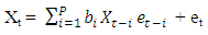 | (1.2) |
Subba Rao (1981) obtained second order moments of the bilinear model BL(p,0,p,1), and Subba Rao and Gabr (1984) obtained third order moments of the BL(1,0,1,1) model. Sessay and SubbaRao (1988, 1991) have also shown that for the BL (p,0,p,1) model, third order moments satisfy Yule-Walker type difference equation.It is well known that the linear autoregressive moving average model can be written in the form of first order vector difference equation (See Anderson, 1971; Priestly, 1978, 1980) and this Vector form is known as the State Space Form. It is convenient to study the properties of a model when it is in the State Space Form (Akaike, 1974). Therefore, we put the pure diagonal bilinear model in the Vectorial form and subsequently examine the conditions under which it is stationary and invertible.
2. Vectorial Representation of the Pure Diagonal Bilinear Model
A time series {Xt} is said to be a diagonal bilinear process if it satisfies the difference equation | (2.1) |
where {et} is a sequence of independent and identically distributed random variables with zero mean and variance  If r = q = 0, the model (2.1) is called Pure diagonal bilinear (PDBL) model and we write it as
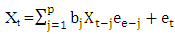 | (2.2) |
where {et} is as defined previously. The model (2.2) is denoted by PDBL (P).Let | (2.3) |
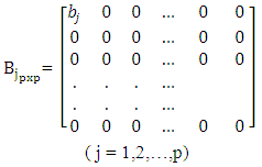 | (2.4) |
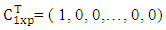 | (2.5) |
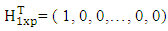 | (2.6) |
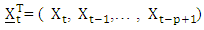 | (2.7) |
where T stands for operation transpose of a matrix. We now represent the model (2.2) in vectorial form.THEOREM 2.1If {Xt} satisfies (2.2) then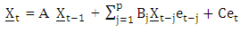 | (2.8) |
is the vectorial form of (2.2)Proof. By direct Verification.
2.1. Stationarity
We want to examine the conditions under which a process {Xt} satisfying (2.8) exists. This type of problem has been tackled by Bhaskara Rao et al (1983) for the special class of models satisfying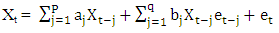 | (2.9) |
After putting this model in vectorial form, they gave a sufficient condition for the existence of a strictly stationary process {Xt} satisfying (2.9). Earlier, Subba Rao and Gabr (1981) gave a sufficient condition for the existence of a second order stationary process {Xt} satisfying (2.9) with P=q. The sufficient conditions in both cases were the same.Subba Rao and Gabr (1981) also obtained the same sufficient conditions for the existence of a second order stationary process {Xt} satisfying | (2.10) |
Under some conditions involving a,b, and  Akamanam et al (1986) have shown that under some conditions on the spectral radius of a matrix, the process {Xt} satisfying (2.1) do exist, are stationary, ergodic and unique.
2.1.1. Vectorial Representaion Method
We now give a set of sufficient conditions under which there is a strictly stationary and ergodic process  satisfying (2.8). We use the methods of Akamanam et al (1986).THEOREM 2.2 (AKAMANAM, BHASKARA RAO, SUBRAMANYAM, 1986)Let {et} be sequence of independent and identically distributed random variables with zero mean and variance
  Let
Let 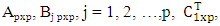
 and
and  be the matrices given by (2.3) to (2.7) respectively.
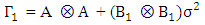

 where
where  is the symbol for Kronecker product of matrices. Suppose all the eigenvalues of the block companion matrix
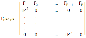 | (2.11) |
have moduli less than unity, where In stands for the identity matrix of order n x n.Then there exists a strictly stationary and ergodic process {Xt} conforming to the model (2.8).Further, if a process {Ut} conforms to the above bilinear model (2.8), then  Proof. See Akamanam et al (1986).
2.1.2. Characteristic Equation Method
We use the above theorem to show that a sufficient condition for the existence of the strictly stationary process {Xt} satisfying (2.2) is that the roots (in modulus) of the characteristic equation | (2.12) |
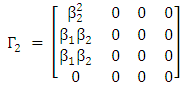
are in absolute value less than unity.We proceed by considering the following cases.CASE 1 P=2 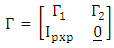 The eigenvalues of
  are obtained as follows:
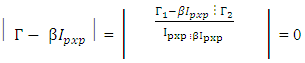 Applying the procedure for obtaining the determinant of a partitioned matrix, we can show that
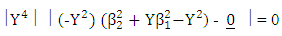
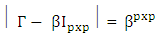
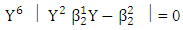
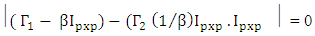 (See Morrison 1976). Simplifying the left-hand side, we have
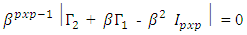 This implies
  since
since  CASE 2 P=3
 Proceeding as in P = 2, we have
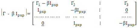
 Simplifying, we have
 This implies that,
  Thus, based on the behavior of the above two cases considered, it can be shown in general that
 Therefore, a sufficient condition for the existence of a strictly stationary process {Xt} satisfying (2.8) is that the roots (in modulus) of the characteristic equation (2.12) are in absolute value less than unity.The following example will illustrate further the work of this section.
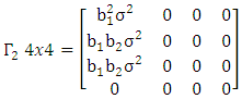 Let
Let  Therefore,
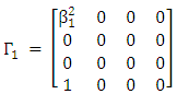
 From case one,
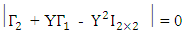 Therefore,
 Implies
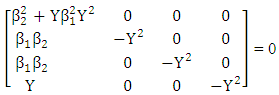 Implies
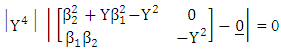
 This implies that
 We have shown that
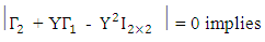
 It is also easy to show that
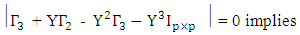
 In general
  Implies
 An alternative approach for obtaining the characteristic equation is given belowTHEOREM 2.3Let {et} be sequence of independent and identically distributed random variable with zero mean and
 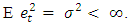 Suppose there exist a stationary and ergodic process {Xt} Satisfying
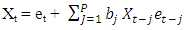 | (2.13) |
Let 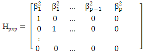 | (2.14) |
Where  Then
Then  Where e(H) is the spectral radius of the matrix H.Proof: Squaring both sides of (2.13) and taking expectations, we obtain
 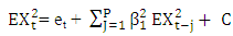 | (2.15) |
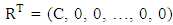
Where Let
Let 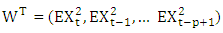
 and H is defined in (2.14). With this notation, we can write (2.13) as the first order difference equation.
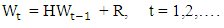 Because of stationarity of {Xt} we have
  for all t. consequently
  This therefore implies that the root (in modulus) of the equation
 | (2.16) |
Lies inside the unit circle.
2.2. Invertibility
For a time series to be useful for forecasting purposes, it is necessary that it should be invertible. We do not know of any nice conditions under which the general bilinear autoregressive moving average model is invertible. The invertibility of special cases of (2.1) have been studied by Granger and Anderson (1978), Subba Rao (1981), Pham and Tran (1981), Quinn (1982) and Iwueze (1988).THEOREM 2.4 (IWUEZE 1988)Let {et} be sequence of independent and identically distributed random variables with E(et) = 0 and  Then the second order strictly stationary and ergodic process {Xt} satisfying
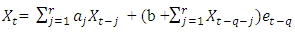 | (2.17) |
for every t is invertible if Iwueze (1988) established that the presence of autoregressive part makes no impact on the invertibility of his special case (2.17).A sufficient condition for invertibility of diagonal bilinear models (2.9) have been derived by Guegan and Pham (1987). It follows that our pure diagonal bilinear model (2.2) is invertible.
2.3. Covariance Structure
The second order properties of various forms of the bilinear model have been shown in the literature to be similar to those of some linear time series models. In particular, the second order covariance structure of the bilinear model BL(P,0,P,1) studied by Subba Rao (1981) is similar to that of an ARMA(P,1) model. Pham (1985) also arrived at the same conclusion after obtaining a Markovian representation of bilinear models. Akamanam (1983) showed that for a special case of the bilinear process, there exists an ARMA process with identical covariance structures.In this section, we show that for every pure diagonal bilinear process (2.2), there exists an ARMA process with identical covariance structure. We give the covariance function in section 2.5.
3. Autocovariances of PDBL(P) Model
It can be shown that for the model (2.2), the following are true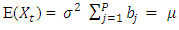 | (2.18) |
 | (2.19) |
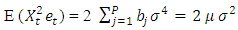 | (2.20) |
 | (2.21) |
 | (2.22) |
We have that the autocovariance function of a stationary process {Xt} is given by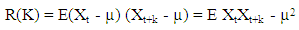 | (2.23) |
Substituting (2.18) and (2.22) into (2.23), we obtain 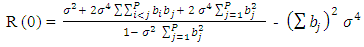 | (2.24) |
Simplifying, we can show that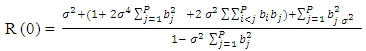 | (2.25) |
Where  Now
Now 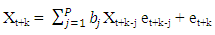 | (2.26) |
Therefore, | (2.27) |
Now, when 
 | (2.28) |
But  | (2.29) |
Therefore, | (2.30) |
Hence, | (2.31) |
Now, for  we have
 | (2.32) |
Therefore, | (2.33) |
Thus, 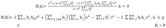 | (2.34) |
This is similar to the autocovariance function of an ARMA(0,P) = MA(P) model. We see that the autocovariance function of a PDBL(P) process like that of a MA(P) process is zero beyond the order P of the process. In other words, the autocovariance function of a PDBL(P) process has a cut off at lag P.
4. Conclusions
In this paper we reviewed the properties of pure diagonal bilinear model. We looked at the conditions under which the pure diagonal bilinear model will be stationary and invertible. We derived the autocovariance function of the pure diagonal bilinear model and observed that it was similar to that of a moving model of order p. This implies that to distinguish between a bilinear model and an ARMA model we have to calculate the autocovariance of the squares of the data.
References
| [1] | AKAIKE H. (1974). Markovian representation of stochastic process and its application to the analysis of autoregressive moving average processes. Ann. Inst. Stat. Math. 26, 336 – 387. |
| [2] | AKAMANAM, S.I. (1983). Some contributions to the study of Bilinear time series models. Unpublished Ph.D. thesis submitted to the University of Sheffield. |
| [3] | AKAMANAM, S.I. BHASKARA RAO, M. AND SUBAMANYAM, K. (1986). On the ergodicity of bilinear time series models. J. time series analysis, 7(3), 157-163. |
| [4] | ANDERSON, T.W. (1971). The statistical analysis of time series. New York and London, Wiley. |
| [5] | BHASKARA RAO, M., SUBBA RAO, T., and WALKER, A.M. (1983). On the existence of some bilinear time series models. J. Time series analysis, 4(2), 95 – 110. |
| [6] | GRANGER, C. W. J. and ANDERSON, A. P. (1978). An introduction to bilinear time series models. Gottingen: Vandenhock and Reprecht. |
| [7] | GUEGAN, D. and PHAM, D. T. (1987). Minimality and inversibility of discrete time bilinear models c.r.a.s., series 1, t. 448, 159 – 162. |
| [8] | IWUEZE, I.S. (1988). On the invertibility of bilinear time series models. To appear is STATISTICA. |
| [9] | MORRISSON, D. F. (1976). Multivariate statistical methods, 2nd ed. Mc Graw – Hill, New York. |
| [10] | PHAM D. T. (1985). Bilinear markovian representation and bilinear models. Stochastic Process Appl. 20, 295 – 306. |
| [11] | PHAM D. T. and TRAN, T.L. (1981). On the first Order Bilinear model. J. Appl. Prob. 18, 617 – 627. |
| [12] | PRIESTLEY, M.B. (1978). Non – linearity in time series analysis. The statistician, 27, 159 – 17. |
| [13] | PRIESTLEY, M.B. (1980). System identification, Kalman filtering and Stochastic Control. In: Directions in Time Series. Institute of Mathematics Statistics, U.S.A. |
| [14] | QUINN, B.G. (1982). Stationarity and invertibility of simple bilinear models. Stochastic Process Applications, 12, 225 – 230. |
| [15] | SUBBA RAO, T. (1981). On the theory of bilinear time series. J.R. Stat. Soc., B, 43, 244 – 255. |
| [16] | SUBBA RAO, T. and GABR, M.M. (1981). The properties of bilinear time series models and their usefulness in forecasting. University of Manchester Institute of Science and Technology. |

 Abstract
 Reference
 Full-Text PDF
 Full-text HTML