-
Paper Information
- Paper Submission
-
Journal Information
- About This Journal
- Editorial Board
- Current Issue
- Archive
- Author Guidelines
- Contact Us
American Journal of Mathematics and Statistics
p-ISSN: 2162-948X e-ISSN: 2162-8475
2016; 6(3): 115-121
doi:10.5923/j.ajms.20160603.05

Convergence of Binomial, Poisson, Negative-Binomial, and Gamma to Normal Distribution: Moment Generating Functions Technique
 Abstract
 Reference
 Full-Text PDF
 Full-text HTML
Subhash C. Bagui1, K. L. Mehra2
1Department of Mathematics and Statistics, University of West Florida, Pensacola, USA
2Department of Mathematical and Statistical Sciences, University of Alberta, Edmonton, USA
Correspondence to: Subhash C. Bagui, Department of Mathematics and Statistics, University of West Florida, Pensacola, USA.
| Email: |  |
Copyright © 2016 Scientific & Academic Publishing. All Rights Reserved.
This work is licensed under the Creative Commons Attribution International License (CC BY).
http://creativecommons.org/licenses/by/4.0/

In this article, we employ moment generating functions (mgf’s) of Binomial, Poisson, Negative-binomial and gamma distributions to demonstrate their convergence to normality as one of their parameters increases indefinitely. The motivation behind this work is to emphasize a direct use of mgf’s in the convergence proofs. These specific mgf proofs may not be all found together in a book or a single paper. Readers would find this article very informative and especially useful from the pedagogical stand point.
Keywords: Binomial distribution, Central limit theorem, Gamma distribution, Moment generating function, Negative-Binomial distribution, Poisson distribution
Cite this paper: Subhash C. Bagui, K. L. Mehra, Convergence of Binomial, Poisson, Negative-Binomial, and Gamma to Normal Distribution: Moment Generating Functions Technique, American Journal of Mathematics and Statistics, Vol. 6 No. 3, 2016, pp. 115-121. doi: 10.5923/j.ajms.20160603.05.
Article Outline
1. Introduction
- The basic Central Limit Theorem (CLT) tells us that, when appropriately normalised, sums of independent identically distributed (i.i.d.) random variables (r.v.’s) from any distribution, with finite mean and variance, would have their distributions converge to normality, as the sample size n tends to infinity. If we accept this CLT and are in knowledge of the fact that Binomial, Poisson, Negative-binomial and Gamma r.v.’s are themselves sums of i.i.d. r.v.’s, we can conclude the limiting normality of these distributions by applying this CLT. We must note, however, that the proof of this CLT is based on the use of Characteristic Functions theory involving Complex Analysis, the study of which primarily only advanced math majors in colleges and universities undertake. There are available, indeed, other methods of proof in specific cases, e.g., in case of Binomial and Poisson distributions through approximations of probability mass functions (pmf) by the corresponding normal probability density function (pdf) using Stirling’s formula (cf., Stigler, S.M. 1986, pp.70-88, [8]; Bagui et al. 2013b, p. 115, [2]) or by simply approximating the ratios of successive pmf terms of the distribution one is dealing with (cf., Proschan, M.A. 2013, pp. 62-63, [6]). However, by using the parallel (to characteristic functions) methodology of mgf’s, which does not involve Complex Analysis, we can also accomplish the same objective with relative ease. This is what we propose to explicitly demonstrate in this paper. The structure of the paper is as follows. We provide some useful preliminary results in Section 2. These results will be used in section 3. In Section 3 we give all the details of convergence for all the above mentioned distributions to normal distribution. Section 4 contains some concluding remarks.
2. Preliminaries
- In this section, we state some results that will be used in various proofs presented in section 3.Definition 2.1. Let
 be a r.v. with probability mass function (pmf) or probability density function (pdf)
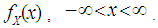 Then the moment generating function (mgf) of the r.v.
  is defined as
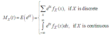 assume to exist and be finite for all
  for an
  If
If  has a normal distribution with mean
  and variance
  , then mgf of
  is given by
 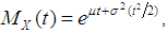 [3]. If
 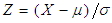 , then
  is said to have standard normal distribution (i.e., a normal distribution with mean zero and variance one). The mgf of
  is given by
  Let
Let  denote the cumulative distribution function (cdf) of the r.v.
  Theorem 2.1. Let
  and
and  be two cumulative distribution functions (cdf’s) whose moments exist. If the mgf’s exist for the r.v.’s
  and
and  and
and  for all
  in
in  then
then  for all
  (i.e.,
  for all
  A probability distribution is not always determined by its moments. Suppose
  has cdf
  and moments
 which exist for all
  . If
. If  has a positive radius of convergence for all
  (Billingsley 1995, Section 30, [4]; Serfling 1980, p. 46, [7]), then mgf exists in the interval
  and hence uniquely determines the probability distribution.A weaker sufficient condition for the moment sequence to determine a probability distribution uniquely is
  This sufficient condition is due to Carleman (Chung 1974, p. 82, [5]; Serfling 1980, p. 46, [7]). Theorem 2.2. Let
  be a sequence of r.v’s with the corresponding mgf sequence as
 and
and  be a r.v. with mgf
  which are assumed exist for all
  If
If  for
for  , then
  The notation
  means that, as
  the distribution of the r.v.
  converges to the distribution of the r.v.
  Lemma 2.1. Let
  be a sequence of reals. Then,
 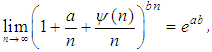 provided
  and
and  do not depend on
  an
an 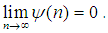 CLT (See Bagui et al. 2013a, [1]). Let
  be a sequence of independent and identically distributed (i.i.d.) random variables with mean
  ,
,  , and variance
  ,
,  , and set
 and
and 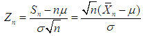 .Then
.Then 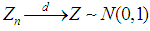 , as
, as  , where
  stands for a normal distribution with mean 0 and variance 1.For Definition 2.1, Theorem 2.1, Theorem 2.2, and Lemma 2.1, see Casella and Berger, 2002, pp. 62-66, [4] and Bain and Engelhardt, 1992, p. 234, [3].
 3. Congergence of Mgf’s
3.1. Binomial
- Binomial probabilities apply to situations involving a series of
 independent and identical trials with two possible outcomes –a success with probability
  and a failure with probability
  - on each trial. Let
  be the number of successes in
  trials, then
  has binomial distribution with parameters
  and
and  . The probability mass function of
  is given by
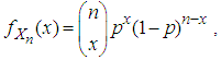
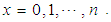 Thus the mean of
  is
is  and the variance of
  is
is 
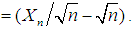
 The mgf of
  is given by
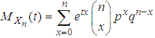
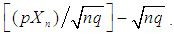
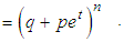 Let
Let 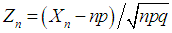 . With simplified notation
 we have
 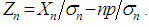 Below we derive the mgf of
  Now the mgf of
  is given by
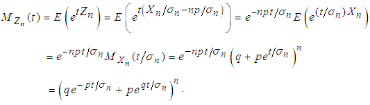 | (3.1) |
 between 0 and
 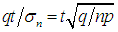 such that
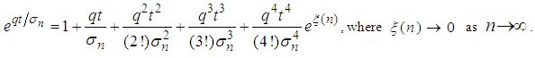 | (3.2) |
 between 0 and
 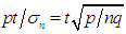 such that
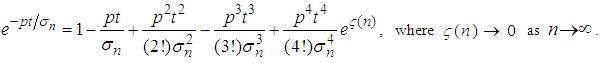 | (3.3) |
 in (3.1), we have
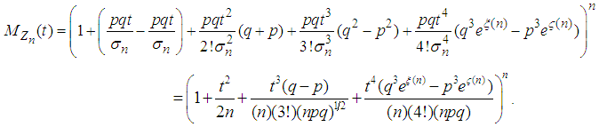 | (3.4) |
 Since
Since 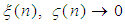 as
as  then
then 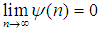 for every fixed value of
  Thus based on Lemma 2.1 we have
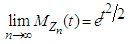 for all real values of
  That is, in view of Theorems 2.1 and 2.2, we conclude that the r.v.
 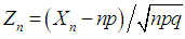 has the limiting standard normal distribution. Consequently, the binomial r.v.
  has, for large
  an approximate normal distribution with mean
  and variance
3.2. Poisson
- The Poisson distribution is appropriate for predicting rare events within a certain period of time. Let
 be a Poisson r.v. with parameter
  The probability mass function of
  is given by
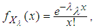
 Both the mean and variance of
  are
are  The mgf of
  is given by
 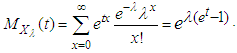 For notational convenience let
  and
and 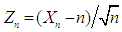
 Below we derive the mgf of
  which is given by
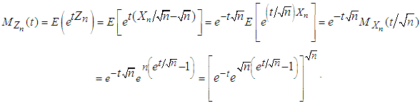 | (3.5) |
 as
as  where
where  is number between
  and
and  and converges to zero as
  Further the above term
  may be simplified as
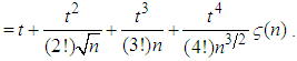 Now substituting this in the last expression (3.5) for
 we have
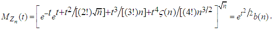 where
where 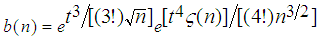 which tends to
  as
as  . Hence, we have
 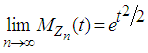 for all real values of
  Using Theorems 2.1 and 2.2 we conclude that
 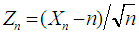 has the limiting standard normal distribution. Hence, the Poisson r.v.
  has also an approximate normal distribution with both mean and variance equal to
  for large
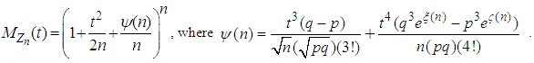
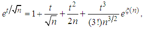
3.3. Negative Binomial
- Consider an infinite series of independent trials, each having two possible outcomes, success or failure. Let
 and
and  Define the random variable
  to be the number of failures before the
  success. Then
  has negative binomial distribution with parameters
  and
and  . Thus, the probability mass function of
  is given by
 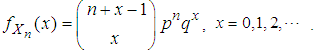 The mean of
  is given by
  and the variance of
  is given by
  The mgf of
  can be obtained as
 Let
Let 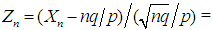
 Now the mgf of
  is given by
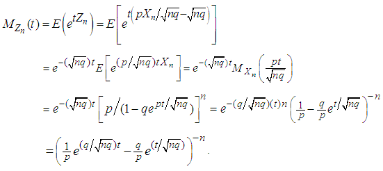 | (3.6) |
 between
  and
and  such that
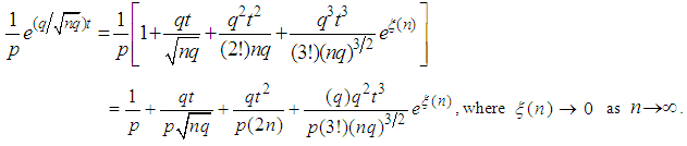 | (3.7) |
 between
  and
and  such that
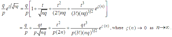 | (3.8) |
 in (3.6), we have
 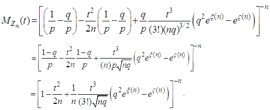 | (3.9) |
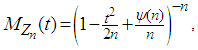 where
where 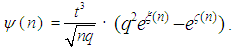 Since both
  as
as  for every fixed value of
  Hence by lemma 2.1 we have
 for all real values of
  Hence, by Theorems 2.1 and 2.2, we conclude the r.v.
  has the limiting standard normal distribution. Accordingly, the negative-Binomial r.v.
  has approximately a normal distribution with mean
  and variance
  for large
3.4. Gamma
- The Gamma distribution is appropriate for modeling waiting times for events. Let
 be a Gamma r.v. with pdf
 and
and  The
The  is called the shape parameter of the distribution and
  is called the scale parameter of the distribution. For convenience let us denote
  by
by  It is well known that the mean of
  is
is  and the variance of
  is
is 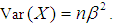 The mgf of
  is given by
  Let
Let 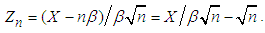 The mgf of
  is given by
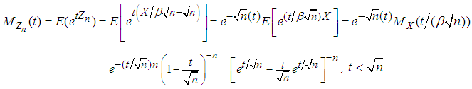 | (3.10) |
 where
where  is a number between
  and
and  and tends to zero as
  and
and 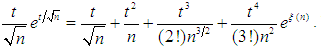 Now substituting these two in the last expression of
  in (3.10), we have
 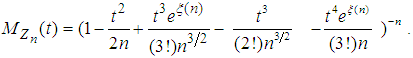 This can be written as
 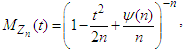 where
where 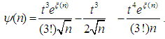 Since
Since  as
as 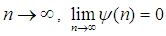 for every fixed value of
  Hence by Lemma 2.1 we have
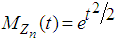 for all real values of
  Hence, by Theorems 2.1 and 2.2, we conclude the r.v.
 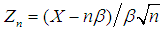 has the limiting standard normal distribution. Accordingly, the Gamma r.v. has approximately a normal distribution with mean
  and varianc
  for large
4. Concluding Remarks
- It is well-known that a Binomial r.v. is the sum of i.i.d. Bernouli r.v.’s, a Poisson
 r.v., with
  a positive integer, the sum of
  i.i.d.
  r. v.’s, a Negative-binomial r.v. the sum of i.i.d. geometric r.v.’s and a Gamma r.v. the sum of i.i.d. exponential r.v.’s. In view of these facts, one can easily conclude by applying the above stated general CLT that the above distributions, after proper normalizations, converge to a normal distribution as
  the number of terms in their respective sums, increases to infinity. But these facts may be beyond the knowledge of undergraduate students, especially those who are non-math majors. However, as demonstrated in the preceding Section 3 for the Binomial, Poisson, Negative-binomial and Gamma distributions, in dealing with distributional convergence problems where individual mgf’s exist and are available, we can use the mgf technique effectively to formally deduce their limiting distributions. In our view, this latter technique is natural, equally instructive and at a more manageable level. In any case, it provides an alternative approach.In the proof of general central limit theorem using mgf both Bain and Engelhardt (1992), [3] and Inlow (2010), [6a] use the mgf of sum of i.i.d r.v’s. But we are using the existing mgf of all the above mentioned distributions without treating them as sums of i.i.d. r.v.’s. Bain and Engelhardt (1992), [3] discusses a proof of convergence of binomial to normal using mgf. But this paper formalizes mgf proofs of collection of distributions. The paper framed in this way can serve as an excellent teaching reference. The proofs are straightforward and require only an additional knowledge of Taylor series expansion, beyond the skills to handle algebraic equations and basic probabilistic concepts. The material should be of pedagogical interest, and can be discussed in classes where only basic calculus and skills to deal with algebraic expressions are the only background requirements. The article should also be of reading interest for senior undergraduate students in probability and statistics.
ACKNOWLEDGEMENTS
- The authors are thankful to the Editor-in-Chief and an anonymous referee for their careful reading of the paper.