1. Introduction

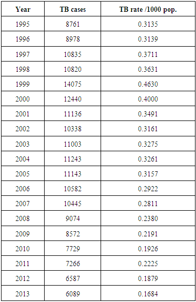
Tuberculosis is an infectious disease and it`s the major cause of morbidity and mortality worldwide, especially in developing countries [1]. Sudan is one of the countries with high TB prevalence. The country has a high burden of tuberculosis TB with an estimated 50,000 incident cases during 2009 [2]. In Sudan 6587 cases had been reported during 2012 [3].

In TB control; Stigma is a major obstacle. Stigmatization of patients renders them to deny the disease and discourage health- seeking services; a behaviour that leads to serious symptoms, non-compliance to treatment and increase the spread of disease [4]. Also this stigma leads to isolation from families, friends, loss of employment, exclusion from the community activities [5], [6]. Studies from different countries; showed that population groups practiced negative attitudes towards TB patients and their families [7], [8], [9].

TB is a large public health problem in Sudan and constitutes a significant burden in primary health care. It is one of the most frequent causes of hospital admissions and hospital related deaths in Sudan. Sudan carries 15% of the TB burden in the Eastern Mediterranean Region (EMR). Sudan is ranked as number three among the highest TB burdened countries in the East Mediterranean Region, and as number two following pakistan in terms of the number of TB patients. In 2010, the estimated incidence of TB cases was 119 per 100 thousand population, to almost 50,000 TB cases. Prevalence of all forms of TB is 209 per 100,000 population or 88,000 cases [10]. The annual risk of TB infection was 1.8 % in 1986 with an estimated number of 90 new smear positive per 100,000 population annually (1986 Sudan national tuberculin survey) [10]. In 1993, the ministry of health in collaboration with the IUATLD and WHO launched formulation of a national wide TB control program (NTP) based on adoption of the DOTS strategy. Since then the program started to expand its infrastructure and established the microscopic network. The NTP reaches its full expansion in 2002 with 300 TB Basic Management Units and 903 DOTS centres [11].

The NTP continued to pursue TB services of good quality that cover completely the northern states of the country. The program sustained valuable microscopic network fully integrated in the Primary health care (PHC) units. However only 35% of the laboratories were subjected to external quality assurance (EQA) in 2006 and maintain adequate supply of good anti TB drugs with standard recording and reporting systems. This was reflected in the good patients’ treatment outcome that the program showed since its establishment. However; an average default rate around 7%has been reported for several years, and not all cases registered for treatment are evaluated. On the other hand, although the program continued to expand its services, it was unable to detect 70% of the estimated TB cases nor to achieve the global target [11]. This is mainly attributed to several gaps and challenges facing the programme as Global TB report data for (2008-2006 notifications). This Study aims at using time series analysis to model quarterly TB cases in Sudan and so to forecast the cases in coming year.

This Study aims at using time series analysis to model quarterly cases of TB cases in Sudan National Tuberculosis program centres to achieve the following objectives: i. Testing the stationarity of the series, ii. Identification of the model that best fit the data, iii. Diagnostic procedure for the model and iv. Estimation of the model.

2. Time Series Models

1. AUTOREGRESSIVE PROCESSES

Assume that a current value of the series is linearly dependent upon its previous value, with some error. Where e_t is a white noise time series. [That is, the e_t are a sequence of uncorrelated random variables (possibly normally distributed, but not necessarily normal) with mean 0 and variance σ²]. This model is called an autoregressive (AR) model, since X is regressed on itself. An autoregressive model (AR) of order p, an AR (p) can be expressed as: [12].

x_t =c + ϕ₁ x_t-1 + ϕ₂ x_t-2 +. . . + ϕ_p x_t-p + et

(1-ϕL– ϕ₂L₂ -... -ϕ_pL_P) x_t = ε_t

Φ (L) X_t = ε_t

2. MOVING AVERAGE PROCESSES (MA)

This is a process that the current value of the series is a weighted sum of past white noise terms, a model like this is called a moving average (MA) model, since X is expressed as a weighted average of past values of the white noise series. Let et (t = 1,2,3,...) be a white noise process, a sequence of independently and identically distributed (I, I, d) random variables with E(et) = 0 and Var(et) = σ² ε. The q^th order of MA model is given as: [12].

xt = m + et + ϴ1et-1 + ϴ2et-2 +. . . + ϴqet-q 87 (1 + Ө1L + Ө2L² + ……+ ӨqL^q)εt = Xt (Lag form)

Φ (L) εt = Xt

3. ARMA PROCESS (p, q)

i. Let e_t be the white noise and X_t the (mixed) Autoregressive Moving Average process of order (p, q) denoted by ARMA (p, q), where n is the number or observation, S is the sample skewness and K is the sample kurtosis. The data comes from a normal distribution if the JB statistic has a chi-square distribution with two degree of freedom. The null hypothesis is that the skewness is zero kurtosis is 3.

ii. Augmented Dickey Fuller (ADF) test: The ADF is a test for unit root in time series samples. It is an augmented version of Dickey Fuller test for a larger and more complicated set of time series models. The ADF test was developed by statisticians D.A Dickey and W. A Fuller (1979).

Where t = p+1, p+2 . . . T

Where α is a constant, β is the coefficient on a time trend and p is the lag order of the autoregressive process. The null hypothesis is that there is a unit root processes against the alternate hypothesis

is the standard error for estimated

The null hypothesis of unit root is accepted if the test statistic is greater than the critical values.

iii. Kwiatkowski, Philips Schmidt and Shin (KPSS) test:

The KPSS test for stationarity Kwiatkowski et al. (1992) tests for stationarity i.e unit root the hypotheses are thus exchanged from those of the ADF test. KPSS type test are intended to complement unit root tests such as Dickey Fuller tests. By testing both the unit root hypothesis and the stationarity hypothesis, one can distinguish between series that appear to have unit root or stationarity. The regression model with a time trend has the form;

y_t = x_t + z_t where x_t is the random walk x_t = x_t-1 + v_t, v_t is independently identically distributed i.e. v_t ~ iid(0,σv) and z_t is the stationary process.

where

The estimate of the long run variance is then give as;

iv. Portmanteau test: The portmanteaus test is used to determine whether or not there is serial correlation in a time series by testing the autocorrelation in the residuals of the model, it tests whether any of a group of autocorrelations of the residual time series are different from zero. The test statistics is; Q=T

Where T is the Sample size, L is the number of autocorrelation lags and ρ (k) is the sample auto correlation at lag k. Under the null hypothesis, the asymptotic distribution of Q is chi-square with L degree of freedom. The null hypothesis is that the series of residuals exhibits no autocorrelation for a fixed numbers of lags L against the alternative hypothesis that some autocorrelation coefficient ρ (k), (k = 1, 2, . . . L) is nonzero. [12]

The Box-Jenkins approach to model building

This section outlines the procedures that Box and Jenkins recommend for constructing a univariate ARIMA model from a given time series. The Box-Jenkins approach to model building follows steps below. The model may then be used to forecast future values.

i. Identification stage

ii. Estimation stage

iii. Diagnostic checking stage

i. Identification stage

Identification is the stage at which a tentative model for the series is selected from the large family of candidate ARIMA (p, d, q) models. Clearly there are many possible combinations of the orders p, d, and q. Thus, the identification stage consists of specifying the AR, I, and MA orders (p, d, q).

ii. Estimation process

Considering an ARIMA (p, d, q) process. A parametric model for the white noise is assumed, this parametric model will be that of Gaussian white noise, then the maximum likelihood is used. We rely on the prediction error decomposition. That is, X_1… X_n have joint density function;

Suppose the conditional distribution of x_t given x₁, . . . , x_t−1 is normal with mean and variance P_t−1, and suppose that x₁~N(1, P₀)

Then for the log likelihood;

Here and P_t−1 are functions of the parameters

Maximum likelihood estimators can be found (numerically) by subtracting −2 log L with respect to these parameters.

iii. Diagnostic checking stage

Once an appropriate model had been entertained and its parameters estimated, the Box Jenkins methodology required examining the residuals of the actual values minus those estimated through the model. If such residuals are random, it is assumed that the model is appropriate. If not, another model is entertained, its parameters estimated, and its residuals checked for randomness [12].

3. Analysis of Data and Interpretation

1. Time plot of TB cases data:

The data plotted above was acquired from National Tuberculosis Program NTP from 1995 – 2013 by quarter TB cases in Sudan. The Plot shows a reduction in the cases there is decreased in TB cases. It also shows a case decline form 2771 case in first quarter in 2007 to 1372 in fourth quarter in 2013. Its annual rate of growth over the period covered is (-0.01389) where that means the TB is decreasing in Sudan in last year’s. And also it can also be seen from the time plot that the data is not stationary and contains trend variation i.e. the mean and variance are not constant and in order to apply certain techniques.

Table (1). Incidents of Tuberculosis in Sudan (1995- 2013)

From the above graphs, show that the time series is likely to have random walk pattern, which random walk up and down in the line graph. Also, in correlogram, the ACFs are suffered from linear decline and there is only one significant spike for PACFs. Then, take the first-difference of TB cases to see whether the time series becomes stationary before further finding AR (p) and MA (q).

Augmented Dickey-fuller (ADF) test for TB cases:

H0: ϕ = 0 (the series yt has a unit root and is non-stationary) versus H1: ϕ < 0 Sample Range: [1994 Q1, 2013 Q4], Total = 72 Asymptotic critical values: 1% 5% 10% -3.524 -2.902 – 2.589 Value of test statistic: -7.418, thus series is said to exhibits unit root since the value of the test statistic is -7.418 is less than the all the critical values.

Correlogram of TB cases:

From the graph of autocorrelation function, it is seen that the series is not stationary in mean and variance because it follows a damped cycle and the PACF suddenly cut off after p lags. The PACF also decline steadily, or follow a damped cycle. Therefore, the series needs to undergo transformation to attain stationarity.

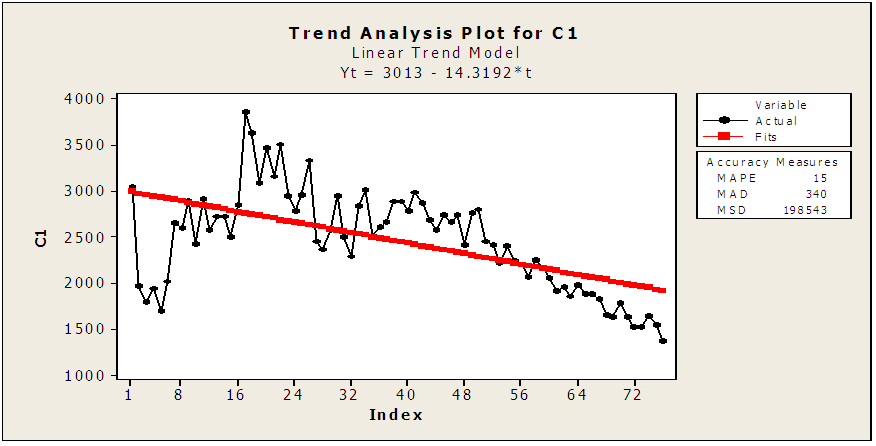Figure (1). Plotting of TB positive cases quarterly (1995- 2013)

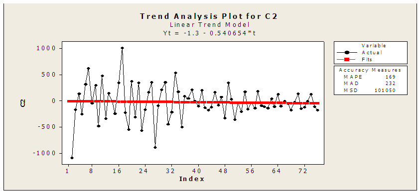Figure (2). Correlogram graph of incidents of TB cases in Sudan (1995-2013)

Time plot of transformed data of TB Cases:

Figure 3 and figure 4 below shows that all ACF and PACF for residuals lies within the intervals, indicating that the model is valid for prediction .The series attains stationarity after taking the first difference i.e the series has a constant mean and finite variance.

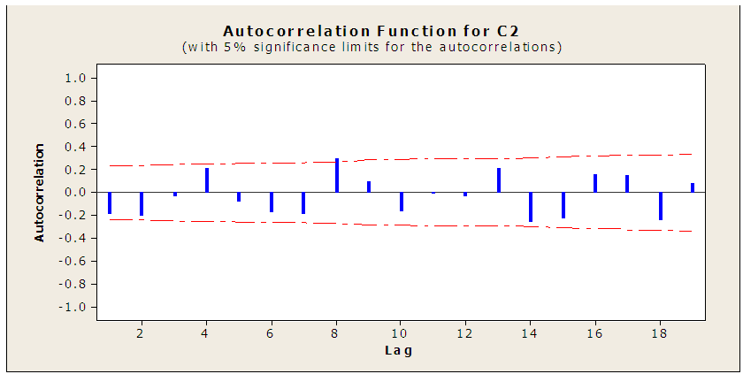Figure (3). Autocorrelation function of TB

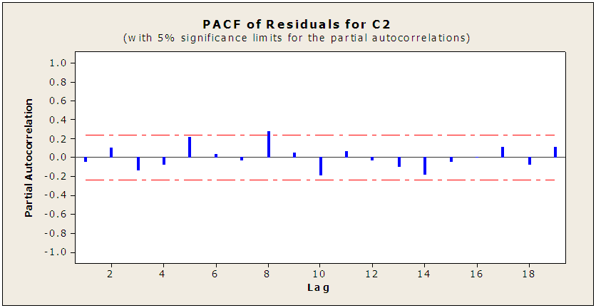Figure (4). ACF of residuals for the series with first difference

Autocorrelation Function: For the series with first difference - C2

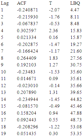Partial Autocorrelation Function: For the series with first difference - C2

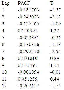Looking to the ACF and PACF for C2 and using Bartlett to determine the P and q values of AR (P) and MA (q) respectively. The calculated value of the test for the nearest correlation in ACF to zero- which is the third value- is "0.12" which is less than the tabulated normal value with 0.05 level of significant "1.96" indicating that the series is stationary at the third lag and hence P = 3. and calculated value of the test for the nearest correlation in PACF to zero -which is the fifth value - is "0.12" which is less than the tabulated normal value with 0.05 level of significant "1.96" indicating that the series is stationary at the fifth lag and hence q = 5. After checking the significant of all possible models, the best model is MA (5):

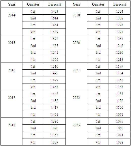
Model diagnostics:

Having seen graphically that the series is stationary in mean and variance from the graph plotted in fig (3), fig (4) and augmented dickey-fuller (ADF) a model has been. Therefore the conclusion is that the ARIMA (0, 1, 1) model is the best-fit ARIMA model for the original time series being analyzed. Using the developed model to forecasting the future cases of TB 2014 – 2023.

Forecasting of TB incidents:

Forecasts of future for cancer cases in Sudan are of particular interest to the in this project work. We may now use the final form of the best-fit ARIMA model for the time series to estimate future cases. The forecasted case for the next three years is displayed Table (2).

Table (2). Forecasting TB cases 2014 – 2023

4. Conclusions

This study examined the prevalence cases of TB in Sudan from 1995 to 2013 using time series methodology. The time plot of the time series of TB cases in Sudan showed that the series has a fairly downward trend pattern which makes the series to be non-stationary and transformed to attain stationarity. Statistical test like ADF and KPSS tests were carried out to confirm the stationarity of the series. After the estimation of the model, it was seen that the ARIMA (0, 1, 1) is appropriate for the model and best fit the model. The forecast suggests an urgent need to curb the menace of the TB minimum, all things being equal.