Poti Abaja Owili1, Dankit Nassiuma2, Luke Orawo3
1Mathematics and Computer Science Department, Laikipia University, Nyahururu, Kenya
2Mathematics Department, Africa International University, Nairobi, Kenya
3Mathematics Department, Egerton University, Private bag, Egerton-Njoro, Kenya
Correspondence to: Poti Abaja Owili, Mathematics and Computer Science Department, Laikipia University, Nyahururu, Kenya.
| Email: |  |
Copyright © 2015 Scientific & Academic Publishing. All Rights Reserved.
Abstract
A major problem facing data analyst is the development and determination of the most efficient imputation technique for imputing missing observations in data used for modeling. Several imputation techniques exist. However, most of them do not take into consideration the probability distribution of the innovation sequence of the time series model. Therefore this study derived optimal linear estimates of missing values for bilinear time series models with GARCH innovations based on minimizing the h-steps-ahead dispersion error. The efficiency of the estimates derived was compared with those obtained using nonparametric techniques of artificial neural network (ANN) and exponential smoothing (EXP) using simulated data. A hundred different samples of size 500 each were generated for two different pure bilinear models with GARCH innovations namely: BL(0,0,1,1) and BL(0,0,2,1). In each sample, artificial missing observations were created at data positions 48, 293 and 496 and estimated using these methods. The performance criteria used to measure the efficiency of these estimates were the mean absolute deviation (MAD) and mean squared error (MSE). The study found mixed results; for the BL(0,0,1,1) model, the optimal linear estimates were the most efficient while for the BL(0,0,2,1), ANN were the most efficient. The study recommends that both ANN and optimal linear estimates be used in estimating missing values for bilinear time series data with GARCH innovations.
Keywords:
Artificial Neural Networks, Exponential Smoothing, Optimal Linear Interpolation
Cite this paper: Poti Abaja Owili, Dankit Nassiuma, Luke Orawo, Efficiency of Imputation Techniques for Missing Values of Pure Bilinear Models with GARCH Innovations, American Journal of Mathematics and Statistics, Vol. 5 No. 5, 2015, pp. 316-324. doi: 10.5923/j.ajms.20150505.13.
1. Introduction
A time series is data recorded sequentially over a specified time period. Data analysts are frequently faced with cases of missing observation at certain points within the data set collected for modeling. Missing values may occur for various reasons which may include poor record keeping, lost records etc. In addition some data, suspected to be outliers, may be deleted because they were erroneously collected. A major problem with missing data is that it can cause havoc in the estimation and forecasting of linear and nonlinear time series as in [2]. Therefore, if data has missing values, it is necessary that the missing value be imputed first before the data is analyzed. Missing value imputation techniques have been developed for several linear and nonlinear time series models. Most of these methods do not consider the distribution of the innovation sequence of the time series data, especially the non-Gaussian distribution. Further, most of these methods only deal with linear ARMA models. In this study, we are interested in a class of nonlinear bilinear time series models whose innovations have GARCH errors. For bilinear time series models, estimation of missing values is still at its infancy stage. This is especially so for bilinear time series models whose innovations are non-Gaussian.A discrete time series process  is said to be a bilinear time series model, denoted byBL (p, q, P, Q), if it satisfies the difference equation
 and
and  and
and  are constant
  and et is the innovation sequence which is normally distributed.For pure bilinear time series model, we have
 It was proposed by Granger and Andersen (1978a) and has been widely applied in many areas such as control theory, economics and finance. For bilinear time series model with GARCH (p, q) innovations, the innovation et is expressed as
 where
where  is a purely random process which is normally distributed. The conditional variance,
  is given by
 In addition, the conditional variance is specified with the inequality conditions:
  for i=1,…,q; and
  , for i=1,…,p to ensure that the conditional variance is strictly positive.A stationary bilinear model can be expressed in a kind of moving average with infinite order as in [7] described by the decomposition theorem. This enhances its application in making inferences. Bilinear models also have the property that although they involve only a finite number of parameters, they can approximate with arbitrary accuracy ‘reasonable’ nonlinearity.Thus far, evaluations of existing implementations of missing values have frequently centered on the resulting parameter estimates of the prescribed model of interest after imputing the missing data. In some situations, however, interest may very well be on the quality of the imputed values at the level of the individual, an issue that has received relatively little attention as in [17]. The basic idea of an imputation approach, in general, is to substitute a plausible value for a missing observation and to carry out the desired analysis on the completed data as in [13]. Here, imputation can be considered to be an estimation or interpolation technique. In this study we were interested in the quality of the estimates of missing values at certain positions in the data. Further, estimates of missing values were derived for pure bilinear time series models with GARCH innovations based on minimizing the h-steps- ahead dispersion error. ANN and exponential smoothing techniques were to obtain estimates of missing values.
2. Literature Review
2.1. Missing Value Imputation: Linear Time Series Models with Finite Variance
Missing values for processes with finite variance have been obtained as in [7]. Reference [15] discussed a method based on forecasting techniques to estimate missing observations in time series. He also compared this method using the minimum mean square estimate as a measure of efficiency based on forecasting techniques to estimate missing observations.Reference [10] discussed two related problems involving time series with missing data. The first concerns the maximum likelihood estimation of the parameters in an ARIMA model when some of the observations are missing or subject to temporal aggregation. The second concerns the estimation of the missing observations. They also pointed out that both problems can be solved by setting up the model in state space form and applying the Kalman filter. Reference [2] applied both methods and demonstrated the superiority of the optimal method.Reference [18] developed a method to find the optimal linear combination of the forecast and back forecast for missing values in a time series which can be represented by an ARIMA model. Reference [7] discussed different alternatives for the estimation of missing observation in stationary time series for autoregressive moving average models. The article offered a series of estimation alternatives for estimating missing observations. Reference [11] demonstrated that missing values in time series can be treated as unknown parameters and estimated by maximum likelihood or as random variables and predicted by the expectation of the unknown values using the given the data. They provided examples to illustrate the difference between these two procedures. It is argued that the second procedure is, in general, more relevant for estimating missing values in time series. Reference [8] also extended the concept of using minimum mean square error linear interpolator for missing values in time series to handle any pattern of non-consecutive observations. Reference [22] later demonstrated a linear recursive technique that does not use the Kalman filter to estimate missing observations in univariate time series. It is assumed that the series follows an invertible ARIMA model. This procedure is based on the restricted forecasting approach, and the recursive linear estimators are obtained when the minimum mean-square error are optimal.Reference [6] extended the method for estimating missing values and evaluating the corresponding likelihood function in scalar time series to the vector cases as in [5]. The series is assumed to be generated by a possibly partially non-stationary and non-invertible vector autoregressive moving average process. It is assumed that no particular pattern of missing data existed.Missing values for linear models with stable innovations have also been considered. Reference [12] developed alternative techniques suitable for a limited set of stable case with index α∈ (1, 2). This was later extended to the ARMA stable process with index α∈ (0, 2] as in [17]. He developed an algorithm applicable to general linear and nonlinear processes by using the state space formulation and applied it in the estimation of missing values.
2.2. Missing Value Imputation: Nonlinear Time Series Models
Reference [13] derived a recursive estimation procedure based on optimal estimating function and applied it to estimate model parameters to the case where there are missing observations as well as handle time-varying parameters for a given nonlinear multi-parameter model. To estimate missing observations, a nonlinear model was formulated which encompasses several standard nonlinear models of time series as special cases as in [2]. It also offers two methods for estimating missing observations based on prediction algorithm and fixed point smoothing algorithm as well as estimating functions equations. Recursive estimation of missing observations in an autoregressive conditional heteroscedasticity (ARCH) model and the estimation of missing observations in a linear time series model are shown as special cases. However, little was discussed with reference to bilinear time series models. The bilinear model used in the study is a very special case of bilinear time series model given by BL(1,0,1,0) where the bilinear term is made of the present innovation only. Reference [10] investigated influence of missing values on the prediction of a stationary time series process by applying Kaman filter fixed point smoothing algorithm. He developed simple bounds for the prediction error variance and asymptotic behavior for short and long memory process. Nonparametric methods have also been proposed for estimating missing observations. When the parameter of interest is the mean of a response variable which is subject to missingness, [3] proposed using the kernel conditional mean estimator to impute the missing values. Time series smoothers estimate the level of a time series at time t as its conditional expectation given present, past and future observations, with the smoothed value depending on the estimated time series model as in [4].Reference [12] derived a recursive form of the exponentially smoothed estimated for a nonlinear model with irregularly observed data and discussed its asymptotic properties. They made numerical comparison between the resulting estimates and other smoothed estimates.Reference [1] used neural networks and genetic algorithms to approximate missing data in a database. A genetic algorithm is used to estimate the missing value by optimizing an objective function.Many other approaches have been developed to recover missing values, such as k-nearest neighbor (KNN) as in [23], least squares imputation as in [22] and least absolute deviation imputation as in [3]. It can be seen from the literature that there are a variety of methods used for estimating missing values in time series models. This is evidence of major interest in this subject area. Further, missing values for nonlinear time series is still at its infancy stage. Estimation of missing values for time series models which are non-Gaussian have not been well tackled. This shows that the literature lacks explicit methods for estimating missing values whose innovations have different probability distributions. One of the techniques which have not been used to derive estimates of missing values for bilinear time series models is the linear interpolation technique and this is discussed below.
2.3. Estimation of Missing Values Using Linear Interpolation Method
Suppose we have one value  missing out of a set of an arbitrarily large number of n possible observations generated from a time series process
  . Let the subspace
  be the allowable space of estimators of
  based on the observed values
  i.e.,
i.e.,  where n, the sample size, is assumed large. The projection of
  onto
onto  (denoted
  ) such that the dispersion error of the estimate (written disp
  is a minimum would simply be a minimum dispersion linear interpolator. Direct computation of the projection
  onto
onto  is complicated since the subspaces
  and
and  are not independent of each other. We thus consider evaluating the projection onto two disjoint subspaces of
  . To achieve this, we express
  as a direct sum of the subspaces
  and another subspace, say
  , such that
  . A possible subspace is
  , where
  is based on the values
  . The existence of the subspaces
  and
and  is shown in the following lemma.
2.4. Lemma
Suppose  is a nondeterministic stationary process defined on the probability space
  . Then the subspaces
  and
and  defined in the norm of the
  are such that
  .Proof:Suppose
  , then
  can be represented as
 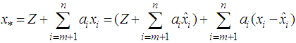 where
where  . Clearly the two components on the right hand side of the equality are disjoint and independent and hence the result. The best linear estimator of
  can be evaluated as the projection onto the subspaces
  and
and  such that disp
 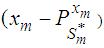 is minimized. i.e.,
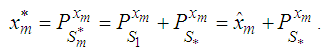 But
But 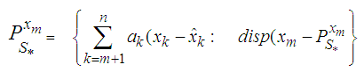 where the coefficients’ are estimated such that the dispersion error is minimized. The resulting error of the estimate is evaluated as
 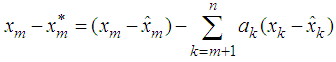 Now squaring both sides and taking expectations, we obtain the dispersion error as
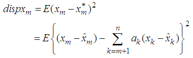 | (1) |
By minimizing the dispersion with respect to the coefficients (differentiating with respect to  and solving for
  ) we should obtain the coefficients
  , for
, for  which are used in estimating the missing value. The missing value
  is estimated as
 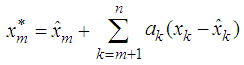 | (2) |
3. Methodology
Three methodologies were used in this study, each corresponding with the estimation method used. These methods included estimation based on optimal linear interpolation, artificial neural network and exponential smoothing. However, the time series data used and performance measures applied were the same for all the methods.
3.1. Methodology for Optimal Linear Interpolation Methods
In this study, the estimators of the missing values for bilinear time series models were derived using optimal linear interpolation method by minimizing the dispersion error. The estimates were derived for pure bilinear time series and general bilinear time series with innovations that have GARCH probability distributions. Estimates of the missing values using non parametric methods were obtained for the artificial neural networks and exponential Smoothing.
3.1.1. Data Collection
Data was obtained through simulation using computer codes written in R-software. Data was generated for the pure bilinear models BL(0,0,1,1) and BL(0,0,2,1).
3.1.2. Missing Data Points
Three data points 48, 293 and 496 selected at random and data at these points removed to create a ‘missing value(s)’ to be estimated at each of these points.
3.1.3. Performance Measures
The MAD (Mean Absolute Deviation) and MSE (Mean Squared Error) were used. These were obtained as follows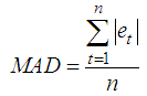 | (3) |
and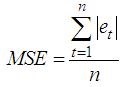 | (4) |
4. Results
4.1. Estimating Missing Values for Bilinear Time Series with GARCH Innovations
These can be computed using the following theorems.
4.1.1. Estimating Missing Values for BL(0,0,1,1) Time Series Model with GARCH Innovations
The simplest pure bilinear time series model of order one, BL(0,0,1,1), is of the form | (5) |
where and
and with the inequality conditions:
  for i=1,…,q,
  , for j=1,…,p to ensure that the conditional variance is strictly positive.Theorem 4.12The optimal linear estimate for missing observation for BL(0, 0,1,1) with GARCH errors is given by
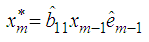 ProofThrough recursive substitution of equation (5), the stationary BL(0,0,1,1) is obtained as
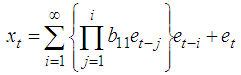 By adding h to t in the equation, the h-steps ahead forecast is
 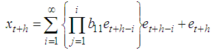 Therefore the forecast error is
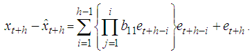 or it can also be represented as
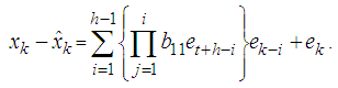 | (6) |
Substituting equation (6) in equation (1), we have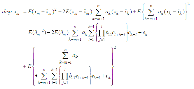 | (7) |
Simplifying each term of equation (7) separately, we have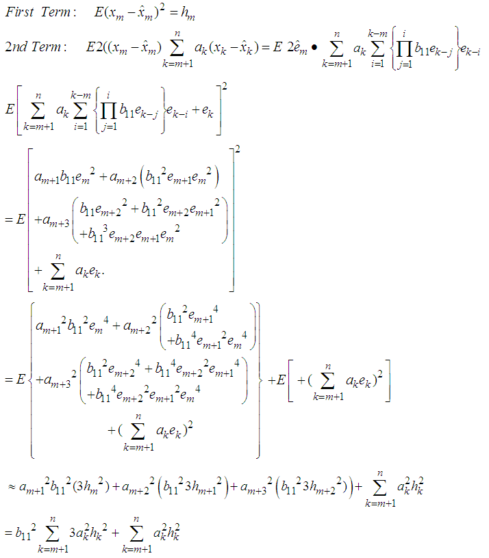 Hence equation (7) can be simplified as
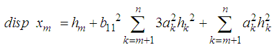 | (8) |
Now differentiating equation (8) with respect to  and equating to zero, we obtain
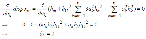 Substituting the values of
  in equation (1), we obtain best estimator of the missing value as
  This shows that the estimate of the missing value is a on step-ahead prediction based on the past observations collected before the missing value. This is in agreement with other studies that have estimated missing values using forecasting as in [24].
4.1.2. Estimating Missing Values for BL (0,0,2,1) with GARCH Innovations
The bilinear time series model with GARCH innovations is given by where
where with the inequality conditions:
  for i=1,…,q,
  , for j=1,…,p to ensure that the conditional variance is strictly positive. Missing values for BL(0,0,2,1) can obtain from the following theorem 4.13.Theorem 4.13 The optimal linear estimate for BL (0,0,2,1) with GARCH errors is given by
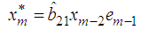 ProofThe stationary BL(0,0,2,1) is given by
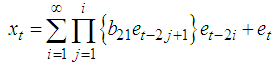 The h-steps ahead forecast error is expressed as
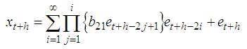 Therefore the forecast error is
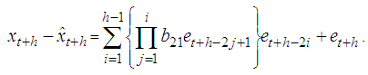 or it can also be represented as
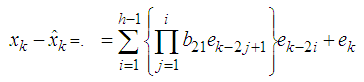 Substituting equation (6) in equation (1), we have
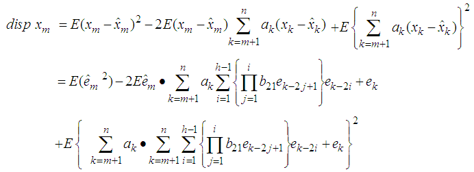 | (9) |
Simplifying each term of equation (9) separately, we have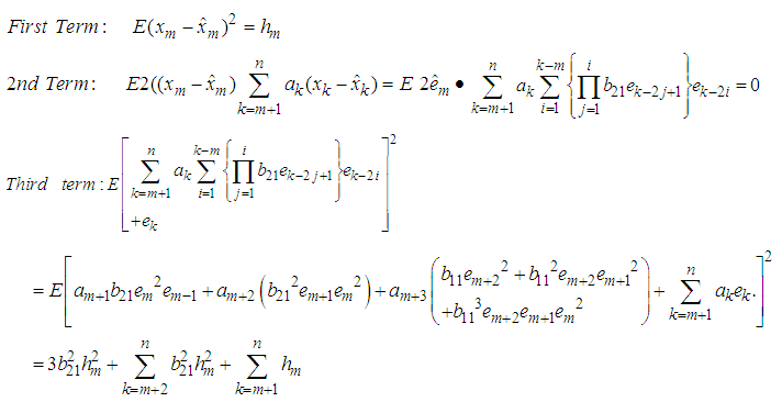 Hence equation (7) can be simplified as
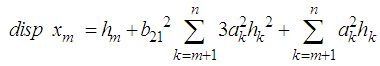 | (10) |
Now differentiating equation (10) with respect to  and equating to zero, we obtain
 Therefore the estimate of the missing value for the BL(0,0,2,1) is
4.2. Simulation Results
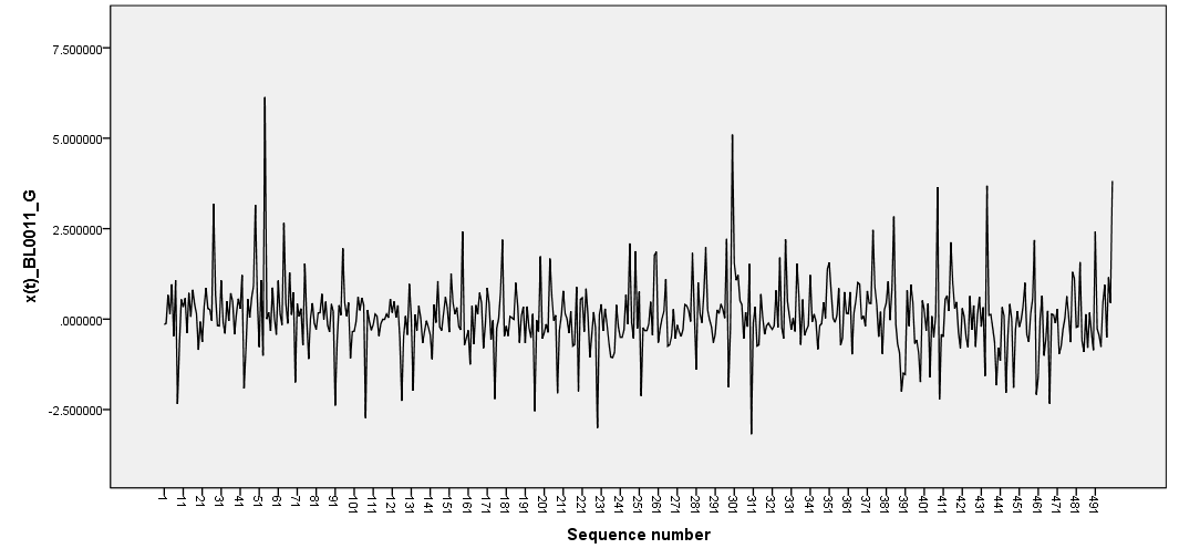
In this section, the results of the estimates obtained for the optimal linear estimate, artificial neural networks and exponential smoothing based on simulated observations from simple pure bilinear models are given. For GARCH distribution the models simulated were BL(0,0,1,1) and BL(0,0,2,1). The R software was used to generate the bilinear random variables. One hundred samples of size 500 were generated for each model and missing values created at positions 47, 293 and 496. The mean absolute deviation (MAD) and mean square error (MSE) were calculated for each model used. Simulation results are given in tables 1 and 2 as well as Figure 1 and 2.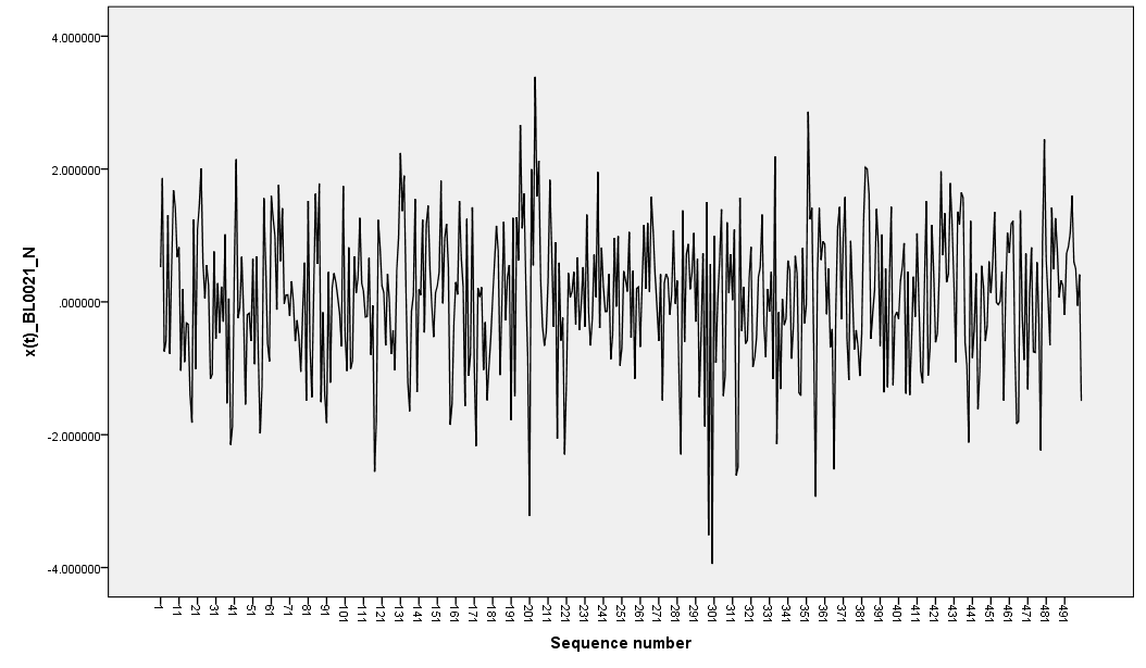 | Figure 1. BL(0,0,2,1) with GARCH(1,1) innovations |
 | Figure 2. BL(0,0,1,1) with GARCH(1,1) innovations |
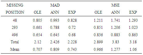
Table 1. Efficiency Measures obtained for GARCH BL(0,0,1,1)
 |
| |
|
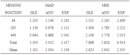
Table 2. Efficiency Measures obtained for GARCH_ Bl(0,0,2,1)
 |
| |
|
The data generated were plotted in graphs as depicted in figure 1 and 2. These graphs are characterized by sharp outburst, clearly evident especially in BL(0,0,1,1). Sharp outburst is one of the characteristics of nonlinearity in bilinear models.Further the study found that when the position of the data was close to the first observation (position 48) then the optimal linear estimates failed to converge on many cases and hence no estimates were recorded. For missing value occurring near the last data in the sample (position 496), the cases of failed convergence were less, about 20%. For most of the cases, estimates based on exponential smoothing were the least efficient. This is discussed below in the following tables.From table 1, it can be observed that estimates based on optimal linear estimates were most efficient (mean=0.7066) for the different missing data point positions followed by EXP smoothing estimates (mean=0.743). Further, the efficiency of the estimates had a negative correlation with the position of the missing value.From table 2, it can be concluded that based on MAD or MSE, the ANN estimates of missing values were the most efficient (mean=1.004) for the different missing data point positions followed by OLE estimates (mean=1.101086).
5. Conclusions
The purpose of this study was to derive the estimates of missing values for pure bilinear time series models with GARCH innovations. The estimates were found to be equivalent to one-step-ahead forecast of the missing value based on the previous observations before the missing value position. The other aim was to compare the efficiency of the estimates obtained using the linear interpolation approach, ANN and exponential smoothing. The study found mixed results. For BL(0,0,1,1) estimates based on optimal linear estimation were the most efficient while for BL(0,0,2,1), estimates based on ANN were more efficient. In both cases estimates based on exponential smoothing were the least efficient. The study recommends that both OLE and ANN techniques should be used for estimating missing values for pure bilinear time series data with missing observations.
5.1. Recommendation for Further Research
A more elaborate research should be done to compare the efficiency of several imputation methods such as K-NN, Kalman filter and estimating functions, genetic algorithms, besides the three used in this study.
Appendix: Program Codes used in Simulation
# The R program (BL1011_GARCH(1,1)b1 <- 0.9; b2<-0.64; s<-0.03; b3<-0.135;b4<- -0.17h<-c()x <-c()e<-c()z<-c()e[1]<- rnorm(1)z[1]<-rnorm(1)h[1]<-c(sqrt(s))x[1]<-c(z[1]*h[1])set.seed(580173)for (i in 2:1500) {e[i] = rnorm(1) # generate noise valuez[i]=rnorm(1)#generates noise valueh[i]= abs(sqrt(s+b2*e[i-1]^2+b3*h[i-1]))x[i] =b4* x[i-1]+b1*x[i-1]*e[i-1]+ z[i]*h[i]}t<- x[-1:-1000]y<-round(t,7)summary(y)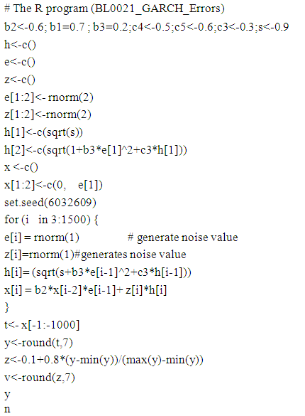
References
| [1] | Abdalla, M.; Marwalla, T. (2005). The use of Genetic Algorithms and neural networks to approximate missing data. Computing and Informatics vol. 24, 5571-589. |
| [2] | Abraham, B.; Thavanesweran, A. (1991). A Nonlinear Time Series and Estimation of missing observations. Ann. Inst. Statist. Math. Vol. 43, 493-504 and Linear lime Series Models. New York,: Springer-Erlag. |
| [3] | Cheng and D. M. Titterington(1994): Neural networks: review from a statistical perspective. Communications in statistics Theory A, 21(12), 3479-3496. |
| [4] | Ledolter, J. (2008). Time Series Analysis Smoothing Time Series with Local Polynomial Regression on Time series. Communications in Statistics—Theory and Methods, 37: 959–971. |
| [5] | Ljung, G. M. (1989). A note on the Estimation of missing Values in Time Series. Communications in statistics simulation 18(2), 459-465. |
| [6] | Luceno, A. (1997). Estimation of Missing Values in Possibly Partially Nonstationary. |
| [7] | Miller, R.B. and Ferreiro,O. (1984). A strategy to complete a time series with missing. |
| [8] | Nassiuma, D. K. (1994). A Note on Interpolation of Stable Processes. Handbook of statistics,Vol. 5 Journal of Agriculture, Science and Technology Vol.3(1) 2001: 81-87. |
| [9] | Nassiuma, D. K. (1994). Symmetric stable sequence with missing observations. J.T.S.A. volume 15, page 317. |
| [10] | Pascal, B. (2005). Influence of missing values on the prediction of a stationary time series. |
| [11] | Pena, D., & Tiao, G. C. (1991). A Note on Likelihood Estimation of Missing Values in Physica D 35 (1989) 395{424. |
| [12] | Pourahmadi, M (1989). Estimation and interpolation of missing values of a stationary time |
| [13] | Thavaneswaran, A.; Abraham (1987). Recursive estimation of Nonlinear Time series models. Institute of statistical Mimeo series No 1835.Time Series. The American statistician, 45(3), 212-213. |
| [14] | Wold, H. (1954). A Study in the Analysis of StationaryTime Series. Almqrist&Wiksell, Stockholm (firstedition 1938). |
| [15] | Abraham, B. (1981). Missing observations in time series. Comm. Statist. A-Theory Methods. |
| [16] | Beveridge, S. (1992). Least Squares Estimation of Missing Values in Time Series.Biometrika, 72, pp. 39-44. |
| [17] | Cortiñas J,A.; Sotto, C;Molenberghs, G; Vromman, G. (2011). A comparison of various software tools for dealing with missing data via imputation. Bart Bierinckx pages 1653-1675. |
| [18] | Damsleth, E. (1979). Interpolating Missing Values in a Time Series. Scand J Statist., 7,data via the EM algorithm,” J. Royal Statist. Soc., ser. B, vol. |
| [19] | Harvey, A. C.; Pierse, R. G. (1984). Estimating missing observations in Economic time series. Journal of the American Association, 79 (385), 125-131. HavardAmerican Journal of Political Science, Vol. 54, No. 2, April 2010, Pp. 561–581C_2010, Midwest Political Science Association. |
| [20] | Nassiuma, D.K and Thavaneswaran, A. (1992). Smoothed estimates for nonlinear time series models with irregular data. Communications in Statistics-Theory and Methods 21 (8), 2247–2259. |
| [21] | Oba S, Sato MA, Takemasa I, et al. A Bayesian missing value estimation method for gene expression profile data. Bioinformatics 2003; 19(16): 2088-2096. |
| [22] | Nieto, F. H., & Martfncz, J. (1996). A Recursive Approach for Estimating Missing Observations in aUnivariate Time Series. Communications in statistics Theory A, 25(9), 2101-2116. |
| [23] | Troyanskaya, O, Cantor, M, Sherlock G, Brown, P, Hastie, T, Tibshirani R, Botstein D and Russ B. Altman1 (2001). Missing value estimation methods for DNA microarrays BIOINFORMATICS Vol. 17 no. 6 2001Pages 520–525. |
| [24] | Granger,. W. J. and Anderse. P. (1978a). Introduction to Bilinear Time Series Models. Gottingen: Vandenhoeck & Ruprecht. |
 Abstract
 Reference
 Full-Text PDF
 Full-text HTML