Abunawas Khaled Abdallah
Department of Mathematics, Qassim University, College of Science and Arts at ArRass, ArRass, Saudi Arabia
Correspondence to: Abunawas Khaled Abdallah, Department of Mathematics, Qassim University, College of Science and Arts at ArRass, ArRass, Saudi Arabia.
| Email: |  |
Copyright © 2015 Scientific & Academic Publishing. All Rights Reserved.
Abstract
In this paper we construct the spline which approximates the function one variable. Spline coefficients are chosen so that the integrals over the domain of the spline function and the same. estimate the error spline. The results of numerical experiments. The use of spline functions in the analysis of empirical two-dimensional data  is described. The definition of spline functions as piecewise polynomials with continuity conditions give them unique properties as empirical functions [2]. They can represent any variation of y with x arbitrarily well over wide intervals of x. Furthermore, due to the local properties of the spline functions, they are excellent tools for differentiation and integration of empirical data. Hence, spline functions are excellent empirical functions which can be used with advantage instead of other empirical functions, such as polynomials or exponentials. [1]
Keywords:
Approximation spline, Function approximation, Estimation error of approximation
Cite this paper: Abunawas Khaled Abdallah, An Approximation Method of Spline Functions, American Journal of Mathematics and Statistics, Vol. 5 No. 5, 2015, pp. 311-315. doi: 10.5923/j.ajms.20150505.12.
1. Introduction
Spline functions are denned as piecewise polynomials of degree n. The pieces join in the so called knots and fulfill continuity conditions for the function itself and the first w - 1 derivatives. Thus a spline function of degree n is a continuous function with n - 1 continuous derivatives.Spline functions have lately found great use as approximating functions in mathematics and numerical analysis; to quote [2] Rice (1969, page 123): "spline functions are the most successful approximating functions for practical applications so far discovered. The reader may be unaware of the fact that ordinary polynomials are inadequate in many situations. This is particularly the case when one approximates functions which arise from the physical world rather than from the mathematical world. Functions which express physical relationships are frequently of a disjointed or disassociated nature. That is to say that their behavior in one region may be totally unrelated to their behavior in another region. Polynomials along with most otherMoreover, since the splines are everywhere represented by simple polynomials, they are computationally easy to handle; their integrals and derivatives are also spline functions, of one degree higher and lower, respectively. Also, the definition of splines in terms of polynomials has the statistically important consequence that a spline function, when fitted to data by least squares, conserves the first two moments of the data [3] (Whittaker 1926, page 307).These nice properties make spline functions excellent also for use in curve fitting in data analysis [3] of observations with random components. However, few applications of splines in this area are found in the literature [4], except for the trivial case of moving averages (which can be seen as splines of degree zero). In our laboratory, spline functions have been used in the analysis of chemical data for some years. The present article reviews my experience with spline functions, specifically as empirical functions used in least squares curve fitting
2. Explanation of Methods
Let a function  ,
,  with the property
 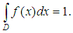 We approximate spline function so that the value of the definite integral on the domain of the function being approximated spline and the same. We use the approximation of a spline defect.On the grid
 spline
  degrees of
  on the segment
  It is expressed by a linear combination of normalized
  - splines:
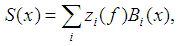 | (1) |
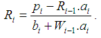
where  – a sequence of linear functional, whose form determines the type of approach.Let us choose
  , so that the value the definite integral at the domain of the function to be approximated, and the spline are equal:
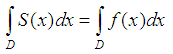 Suppose the domain
  coincides with the segment
  , that is
  ,Then
,Then 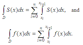 Proceeding from the purposes of the spline, we require that
 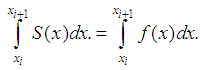 | (2) |
In the interval  the cubic spline
  defect (1) written in the form
 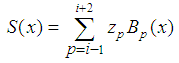 | (3) |
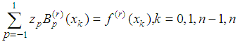
Let us substitute  in the form (3) into the formula (2) and we get to find the coefficients
  system of linear equations
 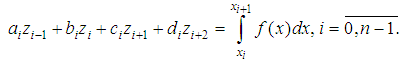 | (4) |
Here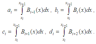 To determine the
  spline coefficients have
  of conditions of the form (2). Additional conditions can be set in a different way, based on knowledge of the properties of the approximated function
  .For example, we require that the value of spline or
  derivative values, respectively, and function or its derivative coincide in three of the four points:
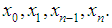
 | (5) |
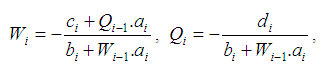
The system (4), (5) has four diagonal matrix of coefficients whose solution will be sought by the sweep method in the form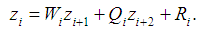
 Consider a function
 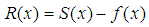 – approximation error. If the function
 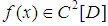 and spline - cubic defect (1), the error
  is a twice continuously differentiable function.
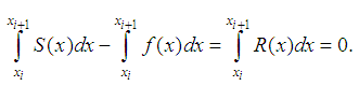 Or
Or From this equation, it follows that
  such that
  , that is for each interval there exists at least one point at which the value of spline
  and the function
  match. We write for
  Taylor formula for the error
 | (6) |
Where . Formula (6), taking into account that
  , each interval can be written as
  . Thus, for the remainder of approximation in the estimate of
  .
. | (7) |
Here  . To construct error estimates of approximation, you can use the following approach. We construct cubic spline
  on points
  , the spline interpolating function for
  , and for the spline
  . At the selected boundary conditions, the following inequality [4]:
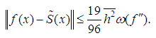 | (8a) |
Here  | (8b) |
For R (x), using the inequalities (8a) and (8b), we construct the evaluation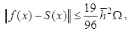 where
where 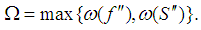 If the mesh is uniform, then the interval
  nonzero
  – splines have the form
 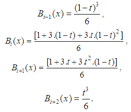 | (9) |
Here 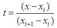 and, taking into account the expressions for
  – splines (9), we obtain
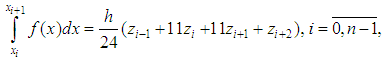 | (10) |
Where  – step uniform grid.We supplement the system (9) by the equations:
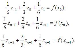 | (11) |
We express from the first equation of the system (11)  substitute in equation (10) for
  and we get the following expression for the
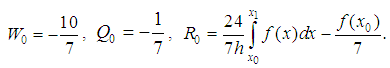 To get a solution at the right boundary introduce the notation
  and write a system of equations on the right border of a
 | (12) |
The first equation of (12) add to (4), enter values  and we get
  equation system (4) as
 We calculate coefficients
  for
for  From the system (12) express
 We consider a spline density distribution, then for a first start time
 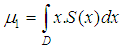 , integrating (1) in the case of equidistant points, we get the expression
 We apply the spline to approximate the probability density function, for example, the standard normal distribution
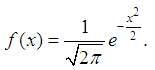 | (13) |
Here  But,
But, 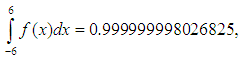 if
if 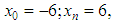 therefore considers the region
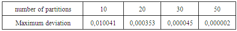
  Table. 1 shows the maximum deviation function
  from the spline
  for the different values of the number of partitions of
  .
.Table 1. Maximum deviation of the function (12) on the values of the spline for any

 |
| |
|
Carried out calculations shown that value of integral of  the region
  deviate from unity by at least
  , While integrals
  calculated to an accuracy of
  . Significance
  , calculated by the formula (11) is equal to zero and with an accuracy of
  . Note that the function (13)
  asymptotically approaching zero, Therefore the method used for verification tasks other conditions present the results, construct a spline for the function
 on the interval
  . The values of the function
  on the borders not equal to zero:
  and
and  , the integral over the area of
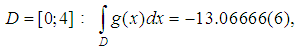
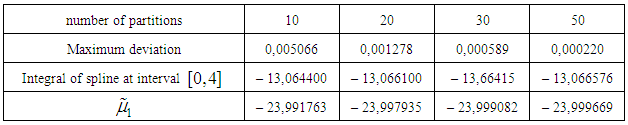
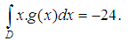 Table. 2 shows the value of the maximum deviation of spline functions
  integral of spline
  and
and 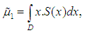 calculated under several
  .
.Table 2. The results of calculations for the function g(x) for different n
 |
| |
|
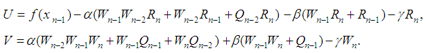
The general solution of differential equations of the fourth order with constant stants coefficients (10)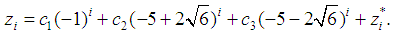 Here
Here  – a particular solution of (10).Consider the application of the proposed spline approximation to the empirical probability density, built at the model data. In [5] It invited the family of linear congruent method for generating base random variable.In general, the linear congruential generator defined by recurrent sequence type
  where
where | (14) |
This sequence is cyclic. According to (14),  so that period of
  . The maximum length of time
  be achieved, it says the following theorem [5].Theorem 1.The maximum possible value of the period sequence (14) and is equal to m if and only if:1)
  and
and  are coprime2)
  multiple of
  for all simple
  is a divisor of
  ,3)
,3)  a multiple of four if
  is a multiple of four.To conduct numerical experiment will use the base generator of the random variable with parameters of
 and
and  and lengths the period
 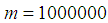 . The method polar coordinates construct a sequence of random numbers having standard normal distribution. Membership used for numerical experiment samples to normal distribution was checked using the agreement criterion
  . [6]Analysis of results numerical experiment showed that spline approximating the empirical distribution shows convergence is the norm of
  – to the the probability density the standard normal distribution (Fig. 1)
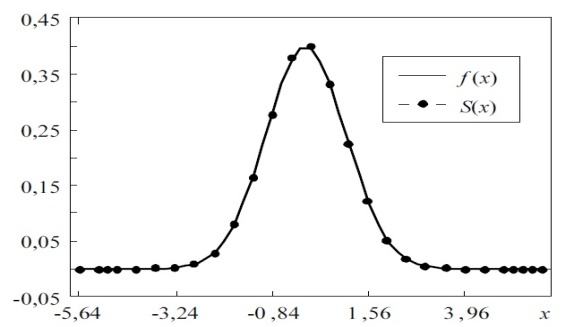 | Figure 1. Spline approximation of the empirical the probability density and timetable density standard normal distribution |
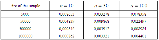
Table. 3 shows the values  , calculated for different
  .
.Table 3. Shows the values
 , calculated for different n , calculated for different n
 |
| |
|
Here  - the probability density function standard normal distribution. By construction of,
  for every partition has a density distribution. By asking increasing number of partitions
  , we get the sequence of functions
  , which deviates from the empirical density on the order of
  , that is with increasing size of the sample and increase the number partitions so that
  , spline function is convergent to the density a standard normal distribution with the second order smallness with respect to
  .
.
3. Conclusions
Spline functions can be used instead of other empirical functions such as polynomials or exponentials for curve fitting of any kind of "continuous" data. Their extreme flexibility and pronounced local properties make them little inclined to introduce bias in the results due to "filtering" effects.* This makes the number of possible applications enormous; the rather simple examples shown in this paper are only a first limited indication of these possibilities [1].It is interesting to note the advantages with the use of empirical spline function descriptions of data even when these are thought to conform well to a theoretical "high information" mathematical model. This description corresponds to a direct investigation of the behavior of the data instead of looking on the data through a sophisticated model. From the applied view, this leads to a higher certainty that the information obtained in the analysis is indeed relevant for the scope of the investigation and does not contain artifacts due to the assumed model. For the theoretician, the spline analysis is an excellent tool for study of the behavior of an accustomed model in relation to the data in question.
References
| [1] | Svante. W. Spline Functions in Data Analysis Technometrics, Vol. 16, No. 1. (Feb., 1974), pp. 1-11. |
| [2] | Rice, J. R. (1969). The approximation of functions, Vol 2. Addison – Wesly, Reading Massachusetts. |
| [3] | Whittaker, E .T. and Robinson G. (1926). The calculus of observations. Blackie and Son Ltd., London. |
| [4] | Zavyalov U. S, Kvassov B. I., Miroshnichenko V. L Methods of spline functions. M.: science, 1980. 352 p. |
| [5] | Knuth D, The Art of Computer Programming: In 3 t. M.: Mir, 1977. T. 2: Seminumerical algorithms. 728. |
| [6] | Larry. Schumaker. Spline Functions: Basic theory;3rd Edition, September 2007. |
 Abstract
 Reference
 Full-Text PDF
 Full-text HTML