Victor Mooto Nawa
Department of Mathematics and Statistics, University of Zambia, Lusaka, Zambia
Correspondence to: Victor Mooto Nawa, Department of Mathematics and Statistics, University of Zambia, Lusaka, Zambia.
| Email: |  |
Copyright © 2015 Scientific & Academic Publishing. All Rights Reserved.
Abstract
An alternative method of estimating parameters in a mixture model for longitudinal trajectories with covariates using the expectation – maximization (EM) algorithm is proposed. Explicit expressions for the expectation and maximization steps required in the parameter estimation of group and covariate parameters are derived. Expressions for the variances of group and covariate parameters for the mixture model are also derived. Simulation results suggest that the proposed approach has good convergence properties especially when covariates are introduced in the model and therefore a good alternative to the current approach which is based on the Quasi-Newton method.
Keywords:
Mixture model, Longitudinal trajectory, PROC TRAJ, Quasi-Newton, EM Algorithm
Cite this paper: Victor Mooto Nawa, A Mixture Model for Longitudinal Trajectories with Covariates, American Journal of Mathematics and Statistics, Vol. 5 No. 5, 2015, pp. 293-305. doi: 10.5923/j.ajms.20150505.10.
1. Introduction
Mixture models have been used in many different fields of study. Closely related to mixture models is the subject of cluster analysis which deals with the search of related observations in a data set. A general methodology for model-based clustering is given by Fraley and Raftery (2002). The application of finite mixture models to heterogeneous data is explained in details in McLachlan and Basford (1988) as well as McLachlan and Peel (2000). Most of the researchers who have studied finite mixture models have used the method of maximum likelihood estimation and the EM algorithm. The EM algorithm (Dempster et al. 1977; McLachlan and Krishnan, 2008) is a general approach for obtaining maximum likelihood estimates for problems in which data can be viewed as incomplete. The basic idea behind the EM algorithm is to frame a given incomplete-data problem into a complete-data problem for which maximum likelihood estimation is computationally tractable. The EM algorithm estimates the parameters of a model iteratively, starting from some initial guess. Each iteration consists of an expectation step (E-step) and a maximization step (M-step).This paper deals with a mixture model for longitudinal trajectories. In particular the paper focusses on the semiparametric group based model proposed by Nagin (1999). This group based model assumes that the population consists of a mixture of distinct groups defined by different trajectory groups. Identifying the different trajectory groups that exist in the population is one of the primary objectives of the modelling strategy. The modelling strategy presumes that two types of variables have been measured: response variables and covariates. Out of the three different data types namely count, binary and psychometric scale data that this modelling approach can handle, we will only concentrate on binary data.Roeder et al. (1999) considered the problem of estimating parameters for this model when response variables and covariates are in the model using the EM algorithm but restricted to count data only. Nawa (2014) considered the problem of estimating parameters in this model based on response variables only using the EM algorithm for longitudinal binary data. This article will consider parameter estimation for a model involving binary longitudinal data based on response variables and covariates using the EM algorithm.Parameter estimates for this modelling approach can be obtained using a SAS procedure called PROC TRAJ written by Jones et al. (2001). This software is a customized SAS procedure that was developed with the SAS product SAS/TOOLKIT. In this SAS procedure, the parameters are obtained by maximum likelihood estimation using the Quasi-Newton method. The results obtained from this procedure are, however, highly dependent on the starting values used (Nawa, 2009). As such, this article presents an alternative approach using the EM algorithm. The remainder of this paper is organised as follows. A brief discussion of mixture models in general and an application to the model under discussion is given in Section 2. This section begins with a discussion of the standard mixture model in Section 2.1. Thereafter a discussion of the longitudinal mixture model with covariates follows in Section 2.2. Section 2.2.1 gives the likelihood formulation of the longitudinal mixture model with covariates clearly outlining the E-steps and M-steps required to estimate the group and the covariate parameters in the model. This is followed by a discussion on estimation of standard errors for the group and covariate parameter values in Section 2.2.2. Simulation results are presented in Section 3 and conclusions are presented in Section 4.
2. The Model
2.1. Standard Mixture Model
A standard mixture model with g groups (McLachlan and Peel, 2000) takes the form | (1) |
where  is a vector of all unknown parameters with
  representing the distribution of group
  and
and  are the unknown mixing proportions where
  are the g groups in the mixture model. If
  is a random sample from the mixture model (1), then the likelihood function for
  can be written in the form
 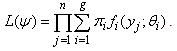 | (2) |
The parameter vector  can be obtained by maximizing the likelihood in (2) or maximizing the log-likelihood given in (3) below.
 | (3) |
Equivalently, the likelihood in (2) can be maximized using the EM (expectation - maximization) algorithm. This is done by maximizing the likelihood in (4) or the log-likelihood in (5) usually referred to as the complete-data log-likelihood  | (4) |
 | (5) |
where  is an indicator variable defined by
2.2. Longitudinal Mixture Model with Covariates
2.2.1. Likelihood Formulation and Parameter Estimation
One of the goals in longitudinal trajectory modelling is to study the effect of risk factors on longitudinal trajectories. The model under investigation has a provision for incorporating the effect of risk factors, time stable and time dependent covariates, on the longitudinal trajectories. Our focus in this paper will just be on the time stable covariates. It is assumed that risk factors affect the likelihood of a particular data trajectory, but nothing more can be learned about the response (Y) from the risk factors (X) given group membership (C) (Jones et al. 2001). Time stable covariates are incorporated in the model by assuming that they influence the probability of belonging to a particular group. Given a sequence  of longitudinal observations measured at m time points on subject j and a set of covariates
  , the likelihood of the joint model based on a sample of n subjects and g groups takes the form
 | (6) |
where  is the probability that the jth subject belongs to group i given the set of covariates x and
  is the probability distribution of the ith group. A polychotomous logistic regression model is used to relate risk factors to group membership and therefore the probability that subject j belongs to group i given a vector of risk factors takes the form
 | (7) |
where  is the jth row of the n by(p+1) matrix of risk factors x and
  is a vector of length (p+1) consisting of covariate parameters associated with group i. Group one is taken as baseline with
  taken as zero and the log odds of membership in group i versus group one are given by
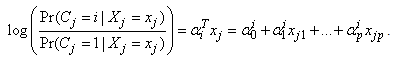 | (8) |
The likelihood in (6) can be equivalently written as  | (9) |
where
 ,
, is a vector of parameters which determines the shape of the trajectory for the ith group and
  is the age of subject j at time t (Nagin, 1999). Since group one is taken as the baseline with
  , the set of all parameters
  is given by
  .The likelihood in (9) can be maximized directly using PROC TRAJ (Jones et al. 2001), however, this paper discusses an alternative way of maximization using the EM – algorithm. Instead of maximizing the likelihood in (9), the EM – algorithm maximizes the complete-data likelihood (or log-likelihood) obtained by introducing an indicator variable
  which takes the value one if the jth observation belongs to group i and zero otherwise. The resulting complete-data likelihood takes the form
 | (10) |
while the complete-data log-likelihood is given by | (11) |
Substituting for  and
and  , the complete-data log-likelihood (11) becomes
 The E-step (expectation step) on the (k+1)th iteration involves evaluating
  , where
  are parameter estimates obtained on the kth iteration. The only random component in the complete-data log-likelihood is
  whose expectation is given by
 | (12) |
Similarly, the M-step on the (k+1)th iteration constitutes finding a value of the parameter vector ψ that maximizes the expected log-likelihood, thus | (13) |
This expected complete-data log-likelihood consists of two sums which can be maximized separately – the first component only depends on the parameter vector  while the second component only depends on the parameter vector
  . In fact, the second component of the expected complete-data log-likelihood can further be separately maximized to obtain
  for each group for
  . Thus we have
 | (14) |
and | (15) |
where  so that
  for
for  . Since there is no closed form solution for
  , the maximization requires iteration. Starting from some initial parameter value
  , the E- and M-steps are repeated until convergence.
2.2.2. Estimation of Standard errors
Standard errors of the parameter estimates can be obtained from the inverse of the observed matrix. The procedure developed by Louis (1982) for extracting the observed information matrix from the complete data log-likelihood when the EM-algorithm is used to find maximum likelihood estimates is used.According to the procedure, the observed information matrix  is computed as
  | (16) |
where | (17) |
is the conditional expectation of the complete-data information matrix  given y and
 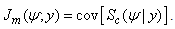 | (18) |
The score vector  based on the complete-data log-likelihood is given by
  | (19) |
where | (20) |
and | (21) |
An expression for  is given in Nawa (2014), thus we only need to find
  . Differentiating the complete-data log-likelihood (11) with respect to
  gives
gives | (22) |
where,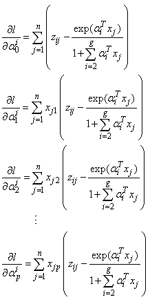 for
for  . Thus,
 ,for
,for  and
and  .The information matrix based on the complete-data log-likelihood (11) can be written as a block-diagonal matrix
  | (23) |
An expression for  is given in Nawa (2014), thus we only need to find
  . The matrix
  can be written as
 | (24) |
where  and
and  (where
  ) are
) are  by
by  matrices respectively given by
 | (25) |
and | (26) |
The  element of the matrix
  is given by
  | (27) |
and | (28) |
for  . Similarly, the
  element of the matrix
  is given by
 | (29) |
and | (30) |
for  .We now find
  , the conditional covariance of the score vector (19). This covariance matrix can be written as
  | (31) |
Expressions for  (for
(for  ) and
) and  (for
(for  ) can be found in Nawa (2014). Therefore we only need to find the other components of the matrix. The covariance matrix
  can be written as
  | (32) |
while  , for
, for  , can be written as
 | (33) |
Let  | (34) |
then | (35) |
and | (36) |
Using (34), (35) and (36), we can show that the (p+1) by (p+1) dimensional matrices  and
and  are respectively given by
 | (37) |
and | (38) |
for  and
and  . Similarly, we can show that the (p+1) by 3 dimensional covariance matrix
  is given by
 | (39) |
and | (40) |
for  and
and  , where
 Putting all the above results together, we can find the expectation of the information matrix based on the complete-data log-likelihood given by
  by finding the expectation of each component of the matrix
  . The matrix
  does not involve
  and is therefore constant with respect to the expectation. The variance estimate for
  is then obtained from the inverse of the matrix
  where the
  in (34) are replaced by the estimated posterior probabilities
3. Simulation Results
We consider simulation results for mixtures of two and three groups of longitudinal trajectories. For a two group model we consider group parameters ,
,  and a covariate parameter
  . For a three group model we consider group parameters
 ,
, ,
,  and covariate parameters
 and
and . Consider a situation involving five time points where measurements are taken at times 1 to 5 (i.e.
  ,
,  ,
,  ,
,  ,
,  ).The group parameter values
 ,
,  and
and  are calculated based on the trajectory shapes given in Figure 1. Using these group parameter values, a sequence of binary responses are independently generated for the time points 1 to 5 with the response from the jth subject of group i at time t being generated with success probability
 | (41) |
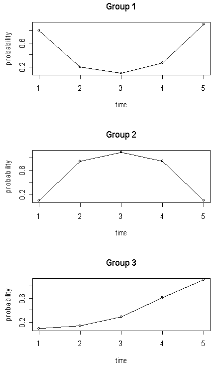 | Figure 1. Longitudinal trajectories for three groups |
In a two group model the covariate parameter is obtained by writing the probability of membership in group 2 as function of x as | (42) |
where  for observations in group 2 and
  for observations in group 1. The values of x and
  are chosen based on a particular value of (42), which is the probability of a subject belonging to group 2.If
  , then x and
  are chosen in such a way that the proportion of ones generated from (42) is equal to
  . Observations for a three group model can be generated in a similar way. Taking group 1 as the baseline
  , we need the probability of belonging to group 2 and the probability of belonging to group 3 as functions of x. These probabilities are respectively given by
 | (43) |
and | (44) |
Taking 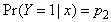 and
and  , we choose x,
  and
and  such that (43) and (44) hold.
3.1. Mixture of Two Trajectory Groups
Consider 150 simulated data sets from a mixture of two trajectory groups with group parameters ,
,  and a covariate parameter
  . For all the 150 simulations, the two methods converged to the same log-likelihood value correct to five decimal places. The mean number of EM steps until convergence was 16.92 while the mean number of iterations for PROC TRAJ was 38.95.Table 1 shows theoretical group parameter values, theoretical covariate parameter values, group parameter estimates, covariate parameter estimates, standard error estimates and empirical standard error estimates obtained from the EM algorithm and the PROC TRAJ procedure. The empirical standard errors reported in the table are sample standard deviations of the actual parameter estimates. Group and covariate parameter estimates obtained from the two methods are very similar and close to the theoretical values. Standard error estimates of the group and covariate parameter estimates obtained from the two methods are also very similar and close to the empirical standard errors. This suggests that the standard error estimates given by the two methods of estimation are a true representation of the variability in the parameter estimates.
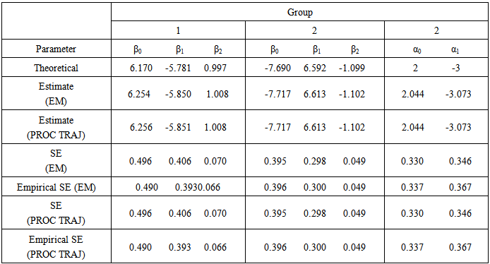 | Table 1. Group parameter estimates, covariate parameter estimates and standard errors based on 150 simulations |
3.2. Mixture of Three Trajectory Groups
Consider 200 simulations from a three group model with group parameters  ,
,  ,
,  and covariate parameters
  and
and  . For all the 200 simulations, the two methods converged to the same log-likelihood value correct to five decimal places. The mean number of EM steps until convergence was 25.11 while the mean number of iterations for PROC TRAJ was 62.16.Table 2 gives the theoretical parameter values, group and covariate parameter estimates obtained from the two methods along with the corresponding standard error and empirical standard error estimates. The table shows that the parameter estimates given by the two methods are almost identical and also very close to the theoretical values. This is true for both the group parameter and covariate parameter estimates. The empirical standard errors are also very close to the estimated standard errors.
 | Table 2. Group parameter estimates, covariate parameter estimates and standard errors based on 200 simulations |
4. Conclusions
This paper is an extension of the work in Nawa (2014), which considered an application of the EM algorithm in estimating group parameters and mixing proportions and the corresponding standard errors in a mixture model of longitudinal trajectories. The paper also compared the results obtained from the EM algorithm to those obtained from the Quasi-Newton method through a SAS procedure called PROC TRAJ proposed by Jones et al. (2001). The extension looks at how the two methods of estimation compare when covariates are introduced in the model. When covariates are introduced in the model, the parameters to be estimated are group parameters and covariates.The paper describes how estimation of various parameters is done using the EM algorithm. Explicit expressions for the expectation steps (E-steps) and maximization steps (M-steps) for each of the parameters are derived. Expressions for computing variances for the parameter estimates are also derived. Most of the expressions are a direct extension of the expressions for the model without covariates.Simulations results indicate that the group parameter estimates, covariate parameter estimates and standard error estimates obtained from the two methods are practically the same. Compared to the model without covariates, parameter estimation in the model with covariates appears to have fewer challenges probably because we have more information separating out the different groups. The simulation results also show that parameter estimates from the model with covariates are also closer to theoretical values compared to the model without covariates. While the EM algorithm seems to have some convergence challenges, especially as the number of groups in the model increases, which is indicated by the number of additional EM steps until convergence to five or more decimal places, this is not the case in the model with covariates. In fact, the number of EM steps until convergence reduces significantly in the model with covariates.The proposed application of the EM algorithm to a model with covariates offers a good alternative to the current method used in the parameter estimation. This is based on the fact that it is known that the current method of estimation is very sensitive to starting values while the EM algorithm is not and from the simulation results that suggest that the convergence seems to improve significantly when the proposed approach is used on a model with covariates.
ACKNOWLEDGEMENTS
I would like to thank Prof K.S. Brown for his invaluable contribution to the work.
References
| [1] | Dempster, A. P., Laird, N. M. and Rubin, D. B. (1977). “Maximum Likelihood for Incomplete Data via the EM Algorithm (with discussion).” Journal of the Royal Statistical Society B, 39, 1 – 38. |
| [2] | Fraley, C. and Raftery, A. E. (2002). “Model-Based Clustering, Discriminant Analysis, and Density Estimation.” Journal of the American Statistical Association, 97, 611 – 631. |
| [3] | Jones, B. L., Nagin, D. S. and Roeder, K. (2001). “A SAS Procedure based on Mixture Models for Estimating Developmental Trajectories.” Sociological Methods and Research, 29, 374 – 393. |
| [4] | Louis, T. A. (1982). “Finding the Observed Information Matrix when using the EM Algorithm.” Journal of the Royal Statistical Society B, 44, 226 – 233. |
| [5] | McLachlan, G. J. and Basford, K. E. (1988). “Mixture Models: Inference and Applications to Clustering.” New York: Marcel Dekker. |
| [6] | McLachlan, G. J. and Krishnan, T. (2008). “The EM Algorithms and Extensions, Second Edition.” New York: Wiley. |
| [7] | McLachlan, G. J. and Peel, D. (2000). “Finite Mixture Models.” New York: Wiley. |
| [8] | Nagin, D. S. (1999). “Analyzing Developmental Trajectories: A Semiparametric Group-Based Approach.” Psychological Methods, 4, 139 – 157. |
| [9] | Nawa, V. M. (2009). “Comparison of the EM algorithm and the Quasi-Newton Method: An Application to Developmental Trajectories.” University of Zambia Journal of Science and Technology, 13 (2), 41 – 54. |
| [10] | Nawa, V. M. (2014). “A Mixture Model for Longitudinal Trajectories”. International Journal of Statistics and Applications, 4 (4), 181 – 191. |
| [11] | Roeder, K, Lynch, K. G. and Nagin, D. S. (1999). “Modelling Uncertainty in Latent Class Membership: A Case Study in Criminology.” Journal of the American Statistical Association, 94, 766 – 776. |
 Abstract
 Reference
 Full-Text PDF
 Full-text HTML