Usoro Anthony E.
Department of Mathematics and Statistics, Akwa Ibom State University, Mkpat Enin, Nigeria
Correspondence to: Usoro Anthony E., Department of Mathematics and Statistics, Akwa Ibom State University, Mkpat Enin, Nigeria.
| Email: |  |
Copyright © 2015 Scientific & Academic Publishing. All Rights Reserved.
Abstract
This paper considered application of linear and bilinear time series models in estimating revenue data. The data used were monthly revenue, which comprised the allocation from Federal Government and internally generated revenue of a Local Government Council in Akwa Ibom State. The motivation behind the comparison between the revenue estimates of linear and bilinear models was to find out if the assertions of [6] and [4] could be applicable to Nigerian system of revenue generation, by using available data at a Local Government level. The aim was to choose more suitable time series model for making projection and proposing feasible targets to revenue generation units or Departments of government establishments. Ordinary least squares method was adopted to estimate the parameters of both linear and bilinear models. From the empirical findings, it was observed that bilinear model fitted the revenue data better than the linear model with standard error difference of 62.66. This affirms the fact that bilinear time series models are more suitable in modeling revenue series, considering the dynamic nature of the time series data. Since the improvement and superiority of bilinear models over linear models are established, this paper recommends forecast of revenue series with bilinear models.
Keywords:
Autoregressive model, Linear model and Bilinear model
Cite this paper: Usoro Anthony E., Comparative Analysis of Linear and Bilinear Time Series Models, American Journal of Mathematics and Statistics, Vol. 5 No. 5, 2015, pp. 265-271. doi: 10.5923/j.ajms.20150505.07.
1. Introduction
In univariate time series, a series is modeled only in terms of its own past values and some disturbance. A particular set of data assumed by a variable, say, Xt, where t represents time, is modeled on the basis of its previous time observations. For instance, every government budget is prepared taking into consideration the past budget figures, be it at the Local, State or Federal Government level. In time series, such expression can be written asXt = f(Xt-1, Xt-2,Xt-3,…,Xt-p, et). The Xt is a variable, which assumes values at the present time period for which forecast can be made, Xt-1, Xt-2,Xt-3,…,Xt-p are the distributed lag variables which represent time past values. The et is the random error assumed to be zero, Johnston and [3]. If, for example, one specified a linear function with one lag and a white noise disturbance, the result would be the first-order autoregressive AR (1) process of the form, Xt = αXt-1 + et.The above model shows that the data series represented by xt is a function of its one period lag. The general form of the model is Xt = α1Xt-1 + α2Xt-2 + α3Xt-3 +,…, + αpXt-p + et. This is a pure autoregressive AR (p) model, with et as a disturbance term. The above model explains the fact, for forecast to be made on the variable, Xt, there must be a relationship between the values of the variable at the present time period and previous time. Therefore, the time series model which expresses such relationship is a linear time series model.In this paper, we also consider bilinear time series model. Bilinear time series model is a model which comprises linear and nonlinear components of the two processes. In time series, the two processes, which make a complete bilinear time series model, are autoregressive and moving average processes. Any of the two processes can be identified in the distribution of autocorrelation and partial autocorrelation functions. For a process to follow autoregressive, the autocorrelation function must exhibit exponential decay or sine wave pattern, while there is a spike or cut- off within the first two lags of partial autocorrelation function. In moving average process, partial autocorrelation function exhibits exponential decay or sine wave pattern, while there is a cut-off or spike within the first two lags of autocorrelation function. These two processes separately form linear model, called AUTOREGRESSIVE MOVING AVERAGE MODEL, ARMA (p,q). In bilinear time series model, there are two parts which make up a complete model. These include linear and nonlinear parts. The nonlinear part is the product of the two processes. Model ‘1’ shown below is an example of a complete bilinear time series model. Model ‘2’ is a complete linear model of autoregressive and moving average processes.
2. Review
The introduction of some nonlinear models, such as logarithmic, quadratic, bilinear time series models to some data is due to the fact that some data assume nonlinearity component. The exhibition of non-linearity property is due to certain occurrences, which some are not under human control. However, there are some events whose occurrences are characterized or generalized by human, but still assume non-linearity. [6] asserted that some of the microeconomic and financial data are not linear due to its dynamic behaviour. According to them, classical linear models are not appropriate for modeling such non-linear series. In most cases, nonlinear forecast is superior to linear forecast. [5] investigated the effect of applying different number of input nodes, activation functions and pre-processing techniques on the performance of back propagation (BP) network in time series revenue forecasting. In the study, several preprocessing techniques were presented to remove the non-stationarity in the time series and their effect on Artificial Neutral Network (ANN) model. The study compared the use of logarithmic function and new proposed Artificial Neutral Network (ANN) model. From the empirical findings, it showed that ANN model, which consisted of small number of inputs and smaller corresponding network structure, produced accurate forecast result although it suffered from slow convergence. [1] reported on the forecast accuracy between time series models and management and analysts. All comparisons were carried out not only on the basis of prediction errors, but also by an analysis of the forecasting bias involved, and the specification of uncertainty. The data used were representative sample of companies listed on the Amsterdam Stock Exchange. The findings revealed improvement on the use of time series models. [4] used a bilinear model to forecast Spanish monetary data and reported a near 10% improvement in one-step ahead mean square forecast errors over several ARMA alternatives.[2] stated the general Bilinear Autoregressive Moving Average model of order (p, q, P, Q) denoted by BARMA (p, q, P, Q) as | (1) |
Xt-i is the distributed lag component of autoregressive process with coefficient αi. Єt-j is the distributed lag component of moving average process with coefficient βj. The sum of the two processes makes up the linear part of model ‘1’. The nonlinear component is the product of the two processes. The model is thus linear in the X’s and also in the Є’s separately, but not in both as product of the two series. In the general ARMA model, | (2) |
Where, the first part on the R.H.S is the autoregressive process, while the second is the moving average process, where Єt is strict white noise,CASE 1: If j = 0, the model becomes | (3) |
This implies  Model 3 is a pure autoregressive model.CASE 2: If i=0, the model becomes
 | (4) |
This implies  Model 4 is a pure moving average model.From model “1”,
 If j=0, the above model becomes
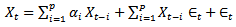 | (5) |
This implies  The model is Bilinear Autoregressive (BAR) model.This is so because the component of the moving average process is eliminated from the general model. The
  in the models is the usual white noise, assumed to be independent and identically distributed with mean zero and variance δe2, [7]. Normally, the values of Єt, being the error values are obtained as deviation of estimates from the original series. Xt is a variable which represents the original values of the revenue series. While, Xt-1, Xt-2, Xt-3… are the time lag of variable Xt.In this paper, we apply Pure Autoregressive (AR) model (3) and Bilinear Autoregressive (BAR) model (5) to fit the revenue data for comparison of estimates between the two models.
3. Method of Estimation
In this paper, the initial process was to obtain the autocorrelation and partial autocorrelation functions of the revenue series, which is represented by Xt. This was done as a procedure to the choice and order of the time series model that is applicable to the data set. The distribution of the autocorrelation function exhibited exponential decay, while partial autocorrelation function indicated a spike at lag 2, as shown in the autocorrelation and partial autocorrelation functions in section ‘3’ below. This distribution suggested autoregressive model of order ‘2’. The model is expresses as Xt = α1Xt-1 + α2Xt-2 + Єt. Єt is the residual, expected to be zero. 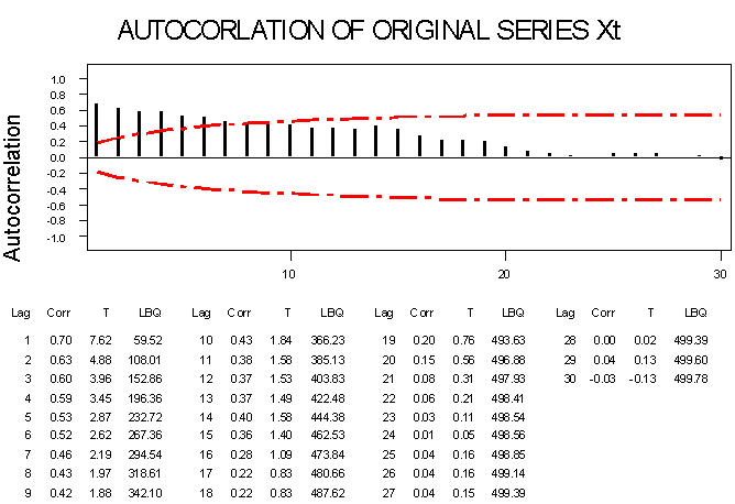 | Figure 1. |
 | Figure 2. |
4. Estimates of Linear and Bilinear Models
Linear Model: From the autocorrelation and partial autocorrelation functions, the revenue series Xt is a function of Xt-1 and Xt-2. This implies the revenue series at the present time period depends on two period lags of itself. Therefore, regression of Xt on Xt-1 and Xt-2 provides the following estimated model for AR (2, 0) process: Xt = 0.603Xt-1 + 0.385Xt-2, where 0.603 and 0.385 are the coefficients of Xt-1 and Xt-2 respectively. The estimated values from the above regression model are the ‘LEXt’ values in the Appendix, and the graphs of the actual and estimates are shown in Time Plot ‘1’.TIME PLOT 1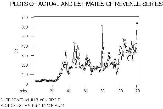 | Figure 3. |
ACF PLOT1 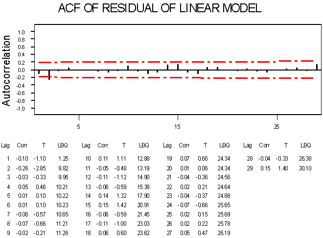 | Figure 4. |
Bilinear Model: This model contains two parts. The linear part, which is the sum of the autoregressive and moving average processes, as shown in the linear model. The second part is always obtained by taking the product of the two processes (autoregressive and moving average processes). But, since the effect of moving average is suppressed as shown the autocorrelation and partial autocorrelation functions, model ‘6’ becomes applicable to the data. The components of the nonlinear part of the model are obtained by taking the products of values of Єt (residual values) and Xt-1 and also Єt and Xt-2 to form Xt-1Єt and Xt-2Єt in the bilinear model, which is expressed as BAR (2, 0, 2, 0). The two zeros in the BAR indicate that both the linear and nonlinear parts of the moving average have zero order. This means the model is a bilinear autoregressive with the order of ‘2’ for the linear and nonlinear parts. The parameters are estimated using ordinary least squares method. Therefore, the regression of Xt on Xt-1, Xt-2, Xt-1Єt and Xt-2Єt produces the following model:Xt = 0.603Xt-1 + 0.422Xt-2 + 0.00113Xt-1Єt + 0.00224Xt-2Єt, where 0.603, 0.422, 0.00113, and 0.00224 are the coefficients of Xt-1, Xt-2, Xt-1Єt and Xt-2Єt respectively. The estimates from the above regression model are the ‘BEXt’ values in the Appendix, and the graphs of the actual and estimates are shown in Time Plot ‘2’.TIME PLOT 2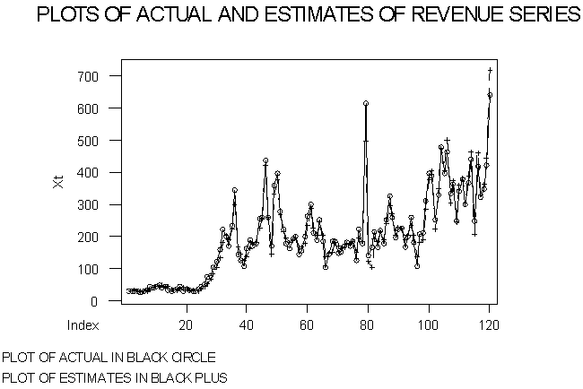 | Figure 5. |
ACF PLOT2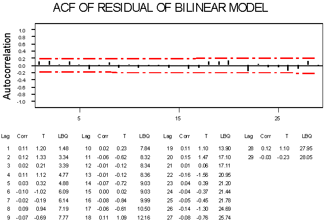 | Figure 6. |
5. Results Interpretation
In fitting the models to the revenue data, autocorrelation and partial-autocorrelation functions were plotted. The distribution suggested autoregressive model of order two. The linear model was estimated, with standard error of 85.51, and the values from the model were plotted on the same graph with the actual data, as shown in Time Plot ‘1’. The ACF Plot ‘1’ is the autocorrelation function of the residual obtained from the estimated linear time series model. From the autocorrelation function, it is observed that there is some level of correlation among the residual values. This correlation implies the residual et is not independent and identically distributed. Secondly, the bilinear model was estimated with standard error of 22.85, and the values from the model were plotted on the same graph with the actual revenue data, as shown in Time Plot ’2’. The ACF Plot ‘2’ is the autocorrelation function of the residual obtained from the estimated bilinear time series model. From the function, it is observed that there is no autocorrelation among the residual values. This explains the fact that the residual et is independent and identically distributed. That is, et is a white noise process, which explains that the bilinear fitted the data set better than linear model.
6. Conclusions
The reason for the application of both linear and bilinear models was to compare the estimates from the two models through the time plot and autocorrelation plots of the two sets of residual values. In time series modeling, one of the aims is to suggest a suitable and best among series of models for estimation and forecast of future values of the observations under consideration. The estimates from the two models have shown that bilinear models are more suitable for the forecast of revenue series.
Appendix
Table of Actual and Estimated Revenue Data
 |
| |
|
References
| [1] | David A. Kodde and Hein Schreuder (1984): Forecasting Corporate Revenue and Profit: Time Series Models Versus Management and Analysts. Journal of Business Finance and Accounting; Volume 11, Issue 3, pages 381-395. DOI.1111/j.1468-5957.1984.tb00757.x. |
| [2] | Granger, C. W. J. and Anderson, A. P. (1978): Introduction to bilinear time series models, Vindenhoeck and Ruprecht. |
| [3] | Johnston, J. and Dinardo, J. (1997): Econometric Methods, McGraw-Hill Companies, Inc, New York. |
| [4] | Maravall, A. (1983): An application of nonlinear time series forecasting. Journal of Business and Economic Statistics; 1, 66-74. |
| [5] | Siti M. Shamsuddin, Roselina Sallehuddin and Norfadzila M. Yusof (2008): Artificial Neutral Network Time Series Modelling For Revenue Forecasting. Chiang Mai Journal of Science; 35(3): 411-426,www.science.cmu.ac.th/journal-science/josci.html. |
| [6] | Subba Rao, T. and Gabr, M. M. (1984): An Introduction to Bispectral Analysis and Bilinear Time Series Models. Lecture Notes on Statistics No. 24 Springer Verlag. |
| [7] | Usoro, A. E. and Omekara. C. O. (2010): Necessary Conditions for Isolation of Special Cases from the General Bilinear Time Series Model. 34th Annual Conference of Nigerian Statistical Association, pp 114 – 117. |
 Abstract
 Reference
 Full-Text PDF
 Full-text HTML