Nabendu Sen , Sanjukta Malakar
Department of Mathematics, Assam University, Silchar
Correspondence to: Nabendu Sen , Department of Mathematics, Assam University, Silchar.
| Email: |  |
Copyright © 2015 Scientific & Academic Publishing. All Rights Reserved.
Abstract
It is found from the literature that most of the authors have considered inventory problems without shortage in fuzzy environment and they also considered different costs as fuzzy numbers and defuzzified by using signed distance method. In our present investigation an attempt has been made to study inventory model with shortage by considering the associated costs involved as fuzzy numbers. In the present piece of work we have referred the work of Dutta and Kumar (2012). They have considered fuzzy inventory model without shortages using trapezoidal fuzzy number and for defuzzification signed distance method was used. Following their work we have extended it for purchasing inventory model with shortages using trapezoidal fuzzy number for different costs and signed distance method for defuzzification, and then for the same purchasing inventory model, the associated costs were considered as different fuzzy numbers like triangular fuzzy number, trapezoidal fuzzy number and parabolic fuzzy number and for defuzzification we have applied Graded Mean Integration Value of defuzzification. Finally numerical illustration has been given. It is observed from this study that the optimal values are improved in fuzzy environment as compared to that of in crisp environment.
Keywords:
Fuzzy Inventory Model, Defuzzification, Optimal Order Quantity
Cite this paper: Nabendu Sen , Sanjukta Malakar , A Fuzzy Inventory Model with Shortages Using Different Fuzzy Numbers, American Journal of Mathematics and Statistics, Vol. 5 No. 5, 2015, pp. 238-248. doi: 10.5923/j.ajms.20150505.03.
1. Introduction
There are many more reasons of maintaining inventories. The proper inventory control help in growth of an organization. The problem of inventory control is broadly associated with answering two questions when to order and how much to order. The problem of making optimal decision with reference to the above two questions is called inventory problem that helps in making decision for minimizing the total cost or maximizing the profit gain. Therefore the solution of inventory problem is a set of specific values of variables under discussion that minimizes the total cost of the system or maximizes the total profit of the system. The objective of many inventory problems is to deal with minimisation of inventory carrying cost (Donalson, 1977). Thus, it is essential to determine a suitable inventory policy to meet the future demand. The basic well known square root formula for EOQ model for constant demand was first given by Haris (1915). Some of the important work done by many researchers like Buchanan (1980), Goyal (1986), Goyel et- al (1986), Hariga (1996), Teng and Thompson (1996). Sarkar and Sana (2010) have developed an inventory model with increasing demand under inflation. In all the above mentioned works, the parameters were taken in crisp environment. However we have found some of the works in inventory management have been done in imprecise environment by considering different parameters as fuzzy numbers and even the demand was also considered as fuzzy demand. Dutta and Kumar (2012) developed fuzzy inventory model without shortages using fuzzy trapezoidal number and used Signed distance method for defuzzification. Yao et al (1999a, 1999b, 2003) considered the fuzzified problem for inventory with or without back order model. Kao and Hsu (2002) consider a single period inventory model with fuzzy demand. Dey and Rawat (2011) proposed an EOQ model without shortage cost by using Triangular fuzzy number and in this case defuzzification was computed by signed distance method. Urgeletti (1983) treated EOQ model in fuzzy sense and used triangular fuzzy number. For different fuzzy numbers and methods of defuzzification, Sen et al (2014) and Dutta and Kumar (2012) were referred.
2. Assumptions and Notations for the Inventory Model in Crisp and Fuzzy Environment
2.1. Assumptions
The following assumptions have been made in this present piece of worki. Demand is deterministic and uniform at a rate D unit of quantity per unit time. Production is instantaneous (i.e., production rate is infinite).ii. Shortage are allowed and fully back logged.iii. Lead time is zero.iv. The inventory planning horizon is infinite and the inventory system involves only one item and one stocking point.v. Only a single order will be produced at the beginning of each cycle and the entire lot is delivered in one batch.vi. C1 be the inventory carrying cost per unit quantity per unit time, C2 be the shortage cost per unit quantity per unit time & C3 be the ordering cost per order, known and constant.vii. Q is the lot-size per cycle whereas S1 is the initial inventory level after fulfilling the back-logged quantity of previous cycle and Q – S1 be the maximum shortage level.viii. T is the cycle length or scheduling period where as t1 be the no shortage period.
2.2. Notations
The following notations are used for developing model in respective environmentC1: carrying cost per unit quantity per unit timeC2: shortage cost per unit quantity per unit timeC3: set up cost per orderT: cycle length or scheduling period D: total demandTC: total costS1: initial inventory level after fulfilling the back logged quantity of previous cycleQ: lot size per cycle Fuzzy carrying cost per unit quantity per unit time
 Fuzzy shortage cost per unit quantity per unit time
 Fuzzy set up cost per order
 Fuzzy total cost
  Optimal order quantityF (S1): defuzzified total costF (S1*): Minimum defuzzified total costetc
3. Mathematical Formulation of Inventory Problems in Different Environments
3.1. Purchasing Inventory Model in Crisp Environment
Regarding the cycle length or scheduling period of the inventory system, two cases may arise: Case I: Cycle length or scheduling period T is constant.Case II: Cycle length or scheduling period T is variable.Case I: In this case, T is constant i.e., inventory is to be replenished after every time period T. As  be the no shortage period,
 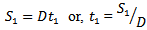 Now, inventory carrying cost during period 0 to
  is
is (Area of ∆ OAB)
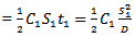
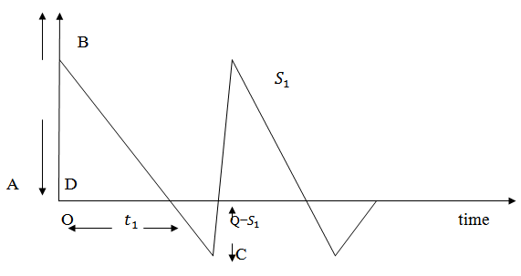 Again shortage cost during the interval
  is
is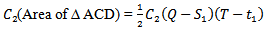
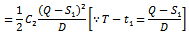 Hence, the total average cost of the system is given by
 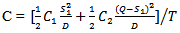 | (3.1) |
Since the set up cost  & time period T are constant, the average set up cost
  also being constant will not be considered in the cost expression.∵ T is constant, Q = DT is also constant. Hence the above expression i.e., the expression for average cost is a function of single variable
  So, we can minimise the above expression with respect to
 | (3.2) |
 | (3.3) |
Case II: In this case, cycle length T is a variable, the average cost of the inventory system will be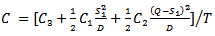 | (3.4) |
Where Q = DTHere the average cost is a function of two independent variables T &  Now for the optimal value of C,
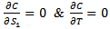 Again
Again  gives
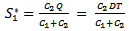
gives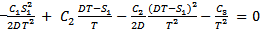 Putting
  in above simplifying we get,
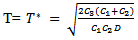 | (3.5) |
Then, 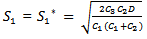 | (3.6) |
Obviously for the value of T &  given
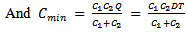
given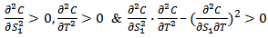 Hence, C is minimum for the value of T &
  ∴ the optimum order quantity for minimum cost is given by
 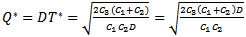 | (3.7) |
 | (3.8) |
3.2. Purchasing Inventory Model in Fuzzy Environment
We consider the model in fuzzy environment. Since the inventory carrying cost and shortage cost, ordering cost are in fuzzy nature, we represent them by trapezoidal fuzzy numbers.Let, Fuzzy carrying cost per unit quantity per unit time
 Fuzzy shortage cost per unit quantity per unit time
 Fuzzy ordering cost per orderCASE 1:Total demand and scheduling period T is constant.The fuzzy total average cost is given by
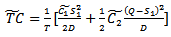 | (3.9) |
Our aim is to apply signed distance method to defuzzify the total average cost and then obtain  by using simple calculus method.Suppose,
 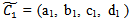 and
and 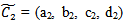 are fuzzy trapezoidal numbers in LR form and a1 , b1, c1 , d1 , a2, b2, c2 , d2 are known positive numbers.From (7.1), we get,
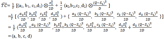 Now,
Now,  Defuzzifying
  by using signed distance method, we have
 | (3.10) |
COMPUTATION OF (S1*) AT WHICH F(S1 ) IS MINIMUM F (s1) is minimum when  and
and 
 Hence,
 Also at s1 = S1*, we have
  This is shown that F(s1 ) is minimum at
  And from (3.10), we find:
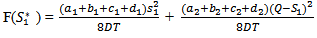 | (3.11) |
Case 2:In this case, cycle length T is a variable, the average total cost of inventory system in fuzzy environment will be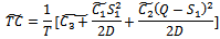 Suppose,
 and
and 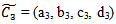 are fuzzy trapezoidal numbers in LR form and from (4), we get,
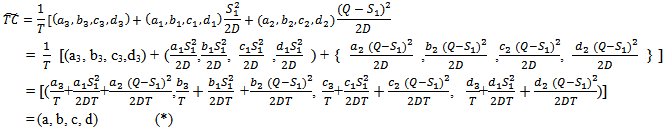 Now,
Now,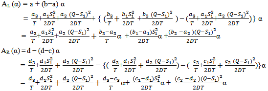 Defuzzifying
  by using signed distance method, we have,
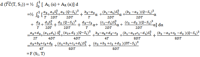 COMPUTATION OF (S1* ) AND T* AT WHICH F(S1,T) IS MINIMUM:For minimum value of F(S1, T), we must have,
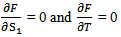 Now,
Now,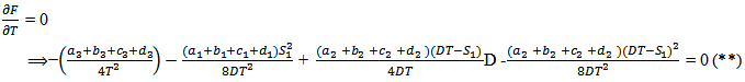 Putting the value of
 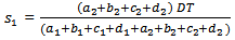 in the above simplifying, we get
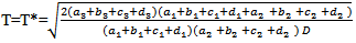 | (3.12) |
Then, 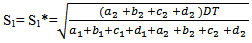 | (3.13) |
Clearly for the value of S1 and T, 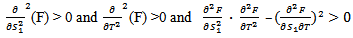 Hence, F (S1, T) is minimum for the value of T and S1.Therefore, the optimal order quantity for minimum cost is given by
 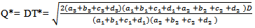 | (3.14) |
 | (3.15) |
3.3. Use of Graded Mean Integration Method for Defuzzification of Different Associated Costs which are Considered Different Fuzzy Numbers
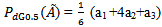
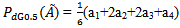
By applying another important method of defuzzification, graded mean integration value of fuzzy numbers we can make study on the same inventory purchasing model whose costs are different fuzzy numbers.By this method of defuzzification:For triangular fuzzy numbers (TFN), 
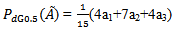
 For parabolic fuzzy numbers (PFN),
 For trapezoidal fuzzy numbers (TrFN),
 In crisp environment:CASE I:Total demand and scheduling period T is constant.
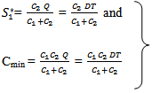 | (3.16) |
CASE II:In this case, cycle length T is a variable.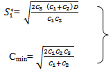 | (3.17) |
In fuzzy environment:For triangular fuzzy number: Suppose, 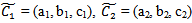 and
and 
 Then,CASE 1:
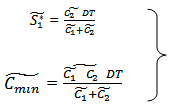 | (3.18) |
CASE 2: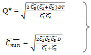 | (3.19) |
For trapezoidal fuzzy number:Suppose, 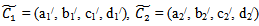 and
and 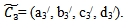 Then,CASE 1:
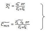 | (3.20) |
CASE 2: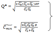 | (3.21) |
For parabolic fuzzy number:Suppose, and
and 
 CASE 1:
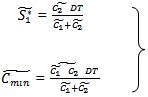 | (3.22) |
CASE 2: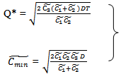 | (3.23) |
Now, to convert the expressions (3.18), (3.19); (3.20), (3.21); (3.22), (3.23) in crisp form, we use graded mean integration method. By this method, the above mentioned expressions (3.18), (3.19); (3.20), (3.21); (3.22), (3.23) reduced to the following form:For triangular fuzzy number: CASE 1: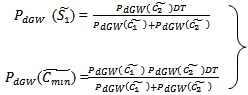 | (3.24) |
CASE 2: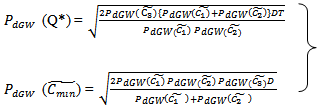 | (3.25) |
For trapezoidal fuzzy number: CASE 1: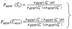 | (3.26) |
CASE 2: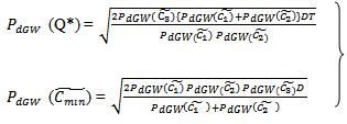 | (3.27) |
For parabolic fuzzy number:CASE 1: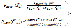 | (3.28) |
CASE 2: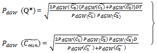 | (3.29) |
Where,For triangular fuzzy number: 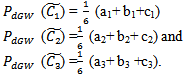 For trapezoidal fuzzy number:
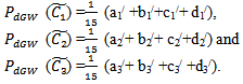 For parabolic fuzzy number:
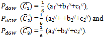
4. Algorithm for Finding Fuzzy Total Cost and Fuzzy Optimal Order Quantity
Step I: Calculate total cost (TC) for the crisp model as given in equation (3.1) and (3.4) for the crisp values of  and D.Step II: Now, determine fuzzy total cost
  using fuzzy arithmetic on fuzzy carrying cost, fuzzy shortage cost and fuzzy ordering cost, taken as fuzzy trapezoidal numbers.Step III: Used Signed distance method for defuzzification. Then, in case I, find
  which can be obtained by putting the first derivative of
  equal to zero and where second derivative of
  is positive at
  And in case II, again we have used signed distance method for defuzzification and using the value of
  we obtained the value of
  Then, find the Fuzzy Optimal order quantity
  which can be obtained by putting the first partial order derivative of
  equal to zero at
  and second partial order derivative of
  is positive at
  and
and  Step IV: Using Graded Mean Integration Method for defuzzification, we find the optimal order quantity
  and
and  for different type of fuzzy numbers, viz. triangular fuzzy number, parabolic fuzzy number and trapezoidal fuzzy number.
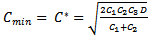
5. Numerical Example
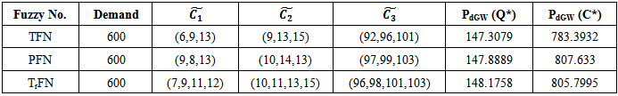
To illustrate the developed model (both in crisp and Fuzzy environment), we have taken an example from Bhunia and Sahoo (2011)In crisp environmentLet, D= 600 units per unit per yearC1= Rs. 10 C2 = Rs. 1 per month C3 = Rs. 100 per order. Then, optimal order quantity Q*= 148 units and the minimum cost per year Cmin=C*= Rs.809.04Table 1. Numerical data for fuzzy valued parameters
 |
| |
|
6. Sensitivity Analysis
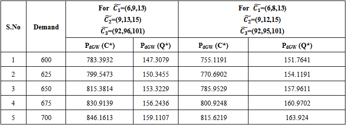
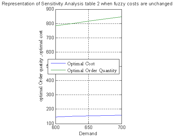
Table 2. Sensitivity Analysis when associated costs are Triangular Fuzzy Number
 |
| |
|
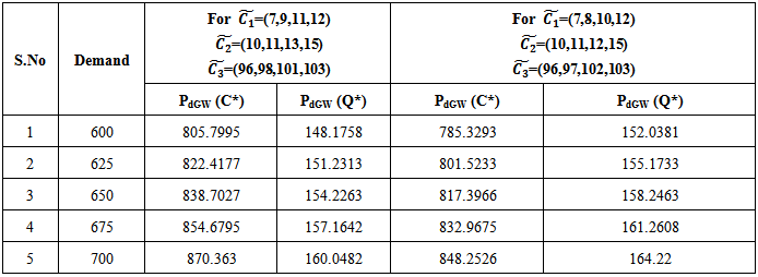
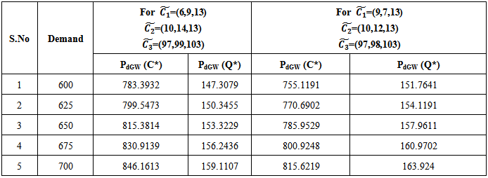
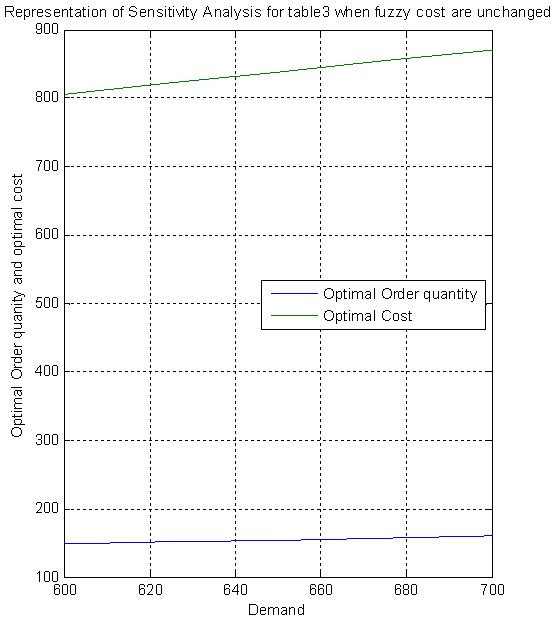
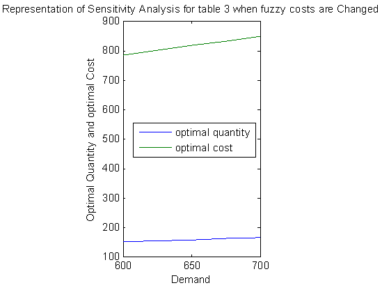
Table 3. Sensitivity Analysis when associated costs are Trapezoidal Fuzzy Number
 |
| |
|
Table 4. Sensitivity Analysis when associated costs are Parabolic Fuzzy Number
 |
| |
|
7. Graphical Representation of Different Results
Similarly the representation of different parameters in table 4 can be made.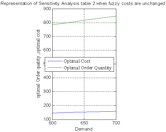
8. Conclusions
Through this investigation, it may be concluded that study of inventory control in fuzzy environment is essential to overcome the imprecision arises in different stages. In reality the cost and demand are not fixed in nature. Different authors have drawn conclusions by considering these as fuzzy numbers. In this study, by considering different costs namely carrying cost, shortage cost and set up cost as different fuzzy numbers and defuzzified by two different defuzzification methods. It is observed that the optimal values are improved as compared to the values in crisp environment. Sensitivity analysis of the results obtained in fuzzy environment helps in making better decision out of number of alternatives. This can further be extended by considering demand as fuzzy numbers and applying fuzzy differential equation. Also, one can apply interval arithmetic for the objective as well as for the parameters involved in different inventory models with shortages. The present study is helpful for business organizations where customers’ demands are not fulfilled instantly.
ACKNOWLEDGEMENTS
Authors are thankful to Dr. A. KBhunia, University of Burdwan and Dr. Biswajit Sarkar, Vidyasagar University for encouragement in developing the interest in the field of Inventory Management. The first author would like to acknowledge the support of UGC-SAP, Mathematics (F.510/5/DRS/2011(SAP-I)), provided by University Grant Commission, New Delhi to Department of Mathematics, Assam University, Silchar.
References
| [1] | Buchanan, J.T. (1980). Alternative solution methods for inventory replenishment problem under increasing demand. Journal of Operational Research Society 31: 615-620. |
| [2] | Bhunia, A.K and Sahoo, L (2011). Advanced Operations Research. Asian Books Private Limited. |
| [3] | Donalson, W.A. (1977). Inventory Replenishment policy for linear trending demand, an analytical solution. Operation research quarterly 28:663-670. |
| [4] | Dutta, D. and Kumar, P. (2012). Fuzzy inventory model without shortage using Trapezoidal Fuzzy number with sensitivity Analysis.IOSR Journal of Mathematics 4:32-37. |
| [5] | Dey, P.K., Rawat A, (2011). A fuzzy inventory model without shortages using triangular fuzzy number.Fuzzy Information and Engineering 1:59-68. |
| [6] | Goyal S.K., (1985). On improving replenishment policies for linear trend demand. Engineering costs and production Economics 10:73-76. |
| [7] | Goyal, S.K., Kusy, M. and Soni, R. (1986). A note on economic order interval for an item with linear trend demand. Engineering costs & Production economics 10: 253-255. |
| [8] | Hariga, M. (1996). Optimal EOQ models for deteriorating items with time-varying demand. Journal of the operational Research Society 47:1228-1246. |
| [9] | Harris, F.W. (1915). Operations and Cost Factory Management Series. USA: A.W. Shaw Co. |
| [10] | Kao, C.K., Hsu, W.K., (2002). A single-period inventory model with fuzzy demand. Computer and Mathematics with application 43:841-848. |
| [11] | Sen, N, Sahoo, L and Bhunia, A.K., (2014). An Application of Integer Linear Programming Problem in Tea Industry of Barak Valley of Assam, India under Crips and Fuzzy Environments. Journal of Information and Computing Science 9(2):132-140. |
| [12] | Sarkar, B., and Sana, S. (2010). A finite replenishment model with increase in demand under inflation. Int, J. Mathematics in Operation research 2(3):347-385. |
| [13] | Teng, J.T and Thompson, G.L. (1996). Optimal strategies for general price quantity decision for new products with learning production costs. European journal of Operational Research 93:476-489. |
| [14] | Urgeletti Tinarelli, G. (1983), Inventory control models and problems.European Journal of General Research 14: 1-12. |
| [15] | Yao, J.S., Lee, H.M. (1999), Economic order quantity in Fuzzy sense for fuzzy order quantity with Trapezoidal fuzzy number.Fuzzy sets and system 105:13-31. |
 Abstract
 Reference
 Full-Text PDF
 Full-text HTML