1. Introduction

Volatility is one of the prime and hidden risk factors on capital markets. Financial time series show random behaviours which is highly unpredictable. Efforts are made to apply the theory of stochastic process and statistical techniques of model building to enhance understanding of apparently, irregular patterns of these financial time series data. Financial time series analysis is concerned with the theory and practice of asset valuation over time. It is a highly empirical discipline but like other scientific fields, theory forms the foundation for making inference. The price of a financial asset evolves over time and forms a stochastic process, which is a statistical term used to describe the evolution of a random variable over time. The observed prices are a realization of the underlying stochastic process. The theory of stochastic process is the basis on which the observed prices are analyzed and statistical inference is made. The price changes can be continuous or discrete. A continuous price can assume any positive real number, whereas a discrete price can only assume a countable number of possible values.

In recent times, nonlinear modeling has received increasing attention in financial time series analysis. These series are affected by a considerable number of sources of nonlinearity such as asymmetrics in the returns, business cycles, asymmetric behaviours of the variability (usually called leverage effect), volatility clustering and so on. These well-known features of financial data imply dynamic behaviours which can be well captured using regime structures. The collection of all random function of a continuous parameter is called a random process. A random process may be uncorrelated, orthogonal and independent of itself. The orthogonality concept is useful only when the random processes under consideration are of zero mean, in this case, it becomes equivalent to the uncorrelated condition. A random process is also stationary when its statistics do not change with the continuous time parameter, that is, it is particularly useful in stationary or purely white noise process. Random processes in continuous time can also be defined as processes with independent increment (standard Weiner process) and processes with independent increment are Markov processes.

The paper is motivated by the recent globalization and increasing complex dependence of financial markets. Financial markets assets depend on a huge number of an underlying of an option such as macro-economic ones like interest rate measurements, foreign currencies, inflation, investments, balanced and unbalanced budgets, micro-economic and business-specific factors like flexibility of labour markets, sales number, etc. Option traders are constantly faced with a dynamically altered volatility risk. Higher risk associated with financial assets requires a risk management and the use of hedging instrument for internationally active organization, Aas [1]. The financial market has become an integral part of the global economy to the extent that any fluctuation in the market influences private and corporate live. In this paper, nonlinear time series is viewed as a realization from stochastic process of a nonlinear dynamical system. Dynamical systems are mathematical objects used to model physical phenomena whose state (or instantaneous description) changes over time. These models are used in financial and economic forecasting; environmental modeling, medical diagnosis, etc.

Applications of dynamical system are broadly categorized into three areas which are predictive in which the objective is to predict future states of the system from observations of the past and present states of the systems. The second is diagnostics, in which the objective is to infer what possibly past states of the system might have led to the present state of the system and finally application, in which the objective is neither to predict the future nor explain the past but rather to provide a theory for the physical phenomena. These three categories correspond to the need to predict, explain and understand physical phenomena. The assumptions in finance for dynamical models are formulated by systems of differential equations. Random dynamical systems are characterized by a state space S, a set of maps T from S into itself that can be thought of as the set of all possible equations of motion and a probability distribution Q on the set T that represents the random choice of map.

2. Literature Review

Many physical processes are continuous in space and time. Any system that depends on the current state is Markovian and follows a diffusion process. The financial system is continuous in space and time just like many physical processes in real life. A stochastic process can be described as a statistical phenomenon that evolves in time according to probabilistic law, Chatfield [4]. The field of stochastic process in continuous time is defined as solutions of stochastic differential equations. Stochastic differential equation is defined as a white noise driven differential equation in which one or more of the terms are stochastic and the solution itself is also a stochastic process. A stochastic process is called Gaussian if all its finite dimensional distribution is multivariate Gaussian. The distribution of a Gaussian stochastic process is determined only by the collection of the expectation and covariance matrices of the finite dimensional distribution, Mikosch [9].

Some established models like the Black-Sholes Options Pricing model have not proven to withstand the test of time and empirical data where stylized features of financial market returns such as volatility clustering, heavy tails and second order serial correlation, etc exist, Dacorogna et al [5]; Bradley and Taqqu [2]. The random level shift model transform data into a linear state space form with a mixture of normal innovations, Li and Perron [8]. The historical (realized) volatility and the implied volatility that are widely used by financial and risk management practitioners are used to determined levels of volatility risk, Forsberg and Bollerslev [6]. Implied volatility is forward looking that reflects the volatility of the underlying assets given its market’s option price. The historical volatility is derived from recent historical data of annualized squared log returns of the option prices observed in the past on the options market, Onyeka-Ubaka et al [10]. Actual market observations conveyed skewness of volatility, i. e. identical option with different strikes possessing different implied volatility. Volatility, standard deviation and risk are sometimes used interchangeably for financial practitioners but in fact there are some conceptual differences, Poon and Granger [12]. The main question is to find out which one of the two market measurements of volatility is better at forecasting true market volatility.

3. Methodology

The model is better viewed as a probability distribution of the stochastic systems in order to capture the dynamics of the system. The methodologies of estimating historical volatility include

(i) Close-Close Volatility Estimator

(ii) High-Low Volatility Estimator

(iii) High-Low-Open-Close volatility Estimator

Suppose a point particle undergoes a one-dimensional, continuous random walk with diffusion constant D. Then, the probability of finding the particle in the interval at time y, if it started at point at time t = 0, is

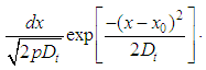By comparison with the normal distribution, we see that D is the variance of the displacement after a unit time interval Parkinson [11]. This suggests the traditional way to estimate D, then, defining = displacement during the i^th interval, 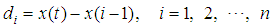, we have the diffusion constant as

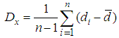as an estimate for D.

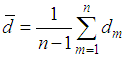= mean displacement

Using this approach, the transformed (logarithmic) price changes, over any time interval in a normally distributed manner with mean zero and variance proportional to the length of the interval and exhibits continuous sample paths. These sample path may be observable anywhere.

Given a series of stock prices 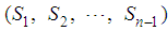which are quoted at equal intervals of a unit of time; equaling

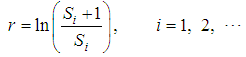
is the mean rate of return, annual number of trading days = 252 days and r is the rate of return over i^th time interval, then the annualized Close-Close estimator, is the classical definition of standard deviation which also happens to be the square root of the diffusion constant definition D. The Close-Close volatility estimator is given as

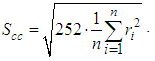This method has some shortcomings such as inadequate usage of readily available information like opening, closing, high and low daily prices in its estimation.

High-Low Volatility Estimator: This is the extreme value method to estimates of variance of the rate of returns. It incorporates the intraday high and low prices of the financial asset into its estimation of volatility. Here the diffusion constant of the underlying random walk of the stock price movements is the true variance of the rate of return of a common stock over a unit of time. The paper established that the use of extreme values in estimating the diffusion constant provides a significantly better estimate.

Let during time interval t and the observed set (l₁, l₂, . . . l_n) originates from a random walk, the factor . The extreme value estimate for the diffusion constant D is

Applying to the stock market, let and the annualized High-Low Volatility Estimator as

High-Low-Open-Close Volatility Estimator: This incorporates not only the high and low historical prices but also the open and closing historical indicators of the stock price movements in estimating variance and hence volatility. The assumptions here were that stock prices follow a geometric Brownian motion. The annualized high-low-open-close volatility estimator (S_HLOC) from Garman and Klass [7] is given as

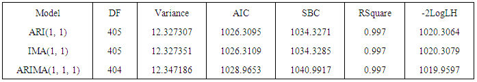
where

O = opening price of the period

C = closing price of the period.

The random variable volatility which is estimated has a tighter sampling distribution.

The model diagnosis was performed. Given a collection of models for the data, Akaike Information Criterion (AIC) estimates the quality of each model, relative to the other models. Hence AIC provides a means for model selection. Let L be the maximized value of the likelihood function for the model; let k be the number of parameters in the model (i.e. k is the number of degrees of freedom). Then the AIC value is as follows

AIC = 2k – 2ln (L)

Given a set of candidate models for the data, the preferred model is the one with the minimum AIC value, hence AIC rewards goodness of fit (as assessed by the likelihood function). It chooses the model with the best fit as measured by the likelihood function, subject to a penalty term to prevent over-fitting that increases with the number of parameters in the model.

4. Results and Discussion

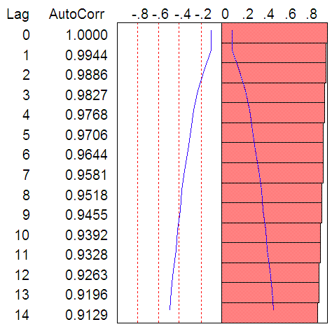
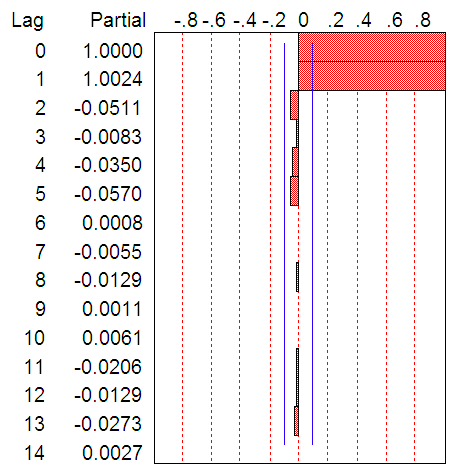
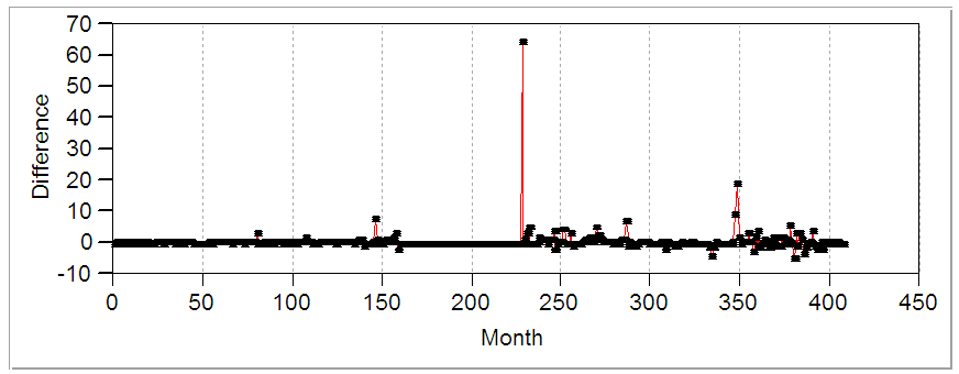
Figure 1 detail plots of the Nigerian Naira to US Dollar exchange rates from 1980 to 2013. The data plotted display a non-stationary pattern with increasing and decreasing behaviour. The autocorrelation function (ACF) and partial autocorrelation function (PACF) decrease slowly indicating non-stationarity of the process. The study adapts the three iterative steps of Box-Jenkins (1976) to select a suitable stochastic model. These steps are identification, estimation and diagnostic checks. The objective of the identification is to select a subclass of the family of autoregressive moving average (ARMA) models appropriated to represent the data. Box-Cox transformation was applied to the data to achieve stationarity in variance while the first difference was used to get the stationarity in mean. The transformed data are plotted in Figure 4. The transformed exchange rates data are both stable and invertible.

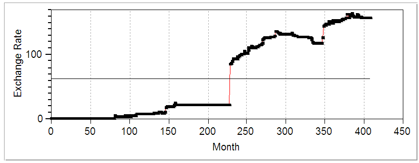Figure 1. Plots of Exchange Rate Data

Figure 2. ACF of Raw Data

Figure 3. PACF of Raw Data

Figure 4. Transformed data (Difference: (1-B)^1)

The graph of Figure 4 shows a series that moves around a constant mean with approximately constant variance. The autocorrelation function (ACF) and partial autocorrelation function (PACF) of the differenced price series are shown in Figures 5 and 6. Figures 5 shows that the series is stationary since the autocorrelation functions is significantly different from zero, indicating a first order moving average type or MA (1). Looking at Figure 6, the partial autocorrelation function is significantly different from zero, indicating a first order autoregressive type or AR (1). But given that the first coefficient show some decreasing structure and lag 4 is statistically significant, perhaps an autoregressive moving average, ARMA (1, 1) model should be tried. The estimation was done with JMPin software. The estimated parameters are presented in Table 1. The model diagnostics were done using Akaike Information Criterion (AIC), Schwartz Bayesian Criterion (SBC), Coefficient of determination (RSquare) and Likelihood Ratio test (-2LogLH). The model with the minimum AIC is selected as the best model that fitted the data.

Table 1. Parameter Estimates and Model Comparison of Exchange Data

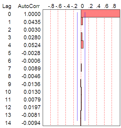Figure 5. ACF of Transformed Data

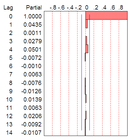Figure 6. PACF of Transformed Data

As shown in the parameter estimates, all the models appear to have statistical strength in terms of the log likelihood ratio test. The models pass the residual diagnostics with very similar results: zero mean hypotheses for the residuals are not rejected and the correlograms indicate that the residuals behave as white noise processes. However, the parameters of the ARIMA (1, 1, 1) models for the products are not statistically significant since the addition of AR term does not seem to improve the results (see the AIC, SBC and R² values in Table 1), we select the more parsimonious ARIMA (1, 1, 0) model as the best for the Naira-Dollar exchange rates during the sampled period (1980-2013). The selected model is used for forecasting. The forecasted exchange rates show that our 95% confidence in the forecasted Naira-Dollar exchange rates are strictly within the lower and upper confidence interval.

Forecasting with an ARI (1) model, the 1-step forecast of Y_T+1 at time T given {Y_T, Y_T-1, . . .} is

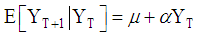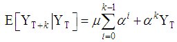The 1-step forecast can be iterated to get the k-step forecast as

As , the forecast approaches the stationary value . The forecast error is given as

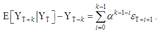The forecast error is therefore a linear combination of the unobservable future shocks entering the system after time T. The variance of the k-step forecast error is given as 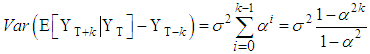Thus, as , the variances increases to the stationary level, .

Forecast

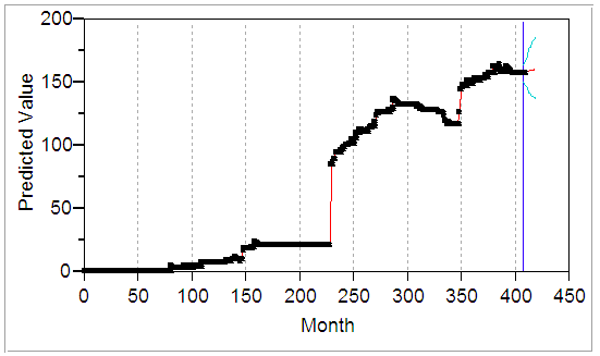Figure 7.

The dashed curves are approximate point wise 95% confidence intervals. As we go further into the future, the forecast approaches the stationary level while the confidence interval widens.

5. Conclusions

The results show that the pricing dynamic of the pricing model is heavily dependent on the dynamic of the underlying stochastic process whether or not the parameters is time varying. Some stylized properties for high frequency exchange market returns such as the non-normal distribution, first order negative autocorrelation, increasing fat tail and seasonality are observed from the analysis. The results establish that using high frequency data improve and outperform volatility forecast performance than the option implied volatility. The paper also establishes that most accurate historical forecasts come from the use of high frequency returns and not from a long memory specification. The forecasted values seem to suggest that the Nigerian economy would be in a dynamical state in which every aspects of the economy would be adversely affected by the steady increase in demand for Dollars. The study therefore calls on stakeholders and Nigerian government in particular to put in place adequate monetary policy to check the dwindling purchasing power of Naira from collapse in the international monetary market.