Imam Akeyede1, Babatunde Lateef Adeleke2, Waheed Babatunde Yahya2
1Department of Mathematics, Federal University Lafia, Lafia, Nigeria
2Department of Statistics, University of Ilorin, Ilorin, Nigeria
Correspondence to: Imam Akeyede, Department of Mathematics, Federal University Lafia, Lafia, Nigeria.
| Email: |  |
Copyright © 2015 Scientific & Academic Publishing. All Rights Reserved.
Abstract
The motivation for this study is that the multi-step forecast performance of nonlinear time series models is often not reported in literature. This is perhaps surprising since one of the main uses of time-series models is for prediction. Therefore, this paper aimed at comparing a number of models that have been proposed in the literature for obtaining h-step ahead forecasts for different features of linear and nonlinear models. These forecasts are compared to those from linear autoregressive model. The comparison of forecasting methods is made using simulations in R software. The relative efficiency of the models was assessed using MSE and AIC criteria. The best model to forecast linear autoregressive function is AR. The performance of LSTAR model supersedes other models as number of steps ahead increases in nonlinear time series data except in polynomial function where SETAR model performs better than others. The predictive ability of the four fitted models increases as sample size and number of steps ahead increase.
Keywords:
SETAR, STAR, LSTAR, MSE, AIC
Cite this paper: Imam Akeyede, Babatunde Lateef Adeleke, Waheed Babatunde Yahya, On Forecast Strength of Some Linear and Non Linear Time Series Models for Stationary Data Structure, American Journal of Mathematics and Statistics, Vol. 5 No. 4, 2015, pp. 163-177. doi: 10.5923/j.ajms.20150504.01.
1. Introduction
The purpose of time series analysis is generally of twofold: to understand or model the stochastic mechanism that gives rise to an observed series and to predict or forecast the future values of a series based on the history of that series and, possibly, other related series or factors. Clements and Smith (2001) evaluated forecasts from SETAR models of exchange rates and compared them with traditional random walk measures. Hansen (2001) used Chow test in testing unknown structural change timing. Boero and Marrocu (2002) showed clear gains from the SETAR model over the linear competitor, on MSEs evaluation of point forecasts, in sub samples characterized by stronger non-linear models. Boero (2003) studied the out-of-sample forecast performance of SETAR models in Euro effective exchange rate. The SETAR models have been specified with two and three regimes, and their performance has been assessed against that of a simple linear AR model and a GARCH model. Kapetanios and Yongcheol (2006) distinguished a unit root process from a globally stationary three-regime SETAR process. Point forecasts are evaluated by means of MSFEs and the Diebold and Mariano test. Interval forecasts are assessed by means of the likelihood ratio tests proposed by Christoffersen (1998), while the techniques used to evaluate density forecasts are those introduced by Diebold et al. (1998). For the evaluation of density forecasts, the modified version of the Pearson goodness-of-fit test and its components is also used, as proposed by Anderson (1994) and recently discussed in Wallis (2002). These methods provide information on the nature of departures from the null hypothesis, with respect to specific characteristics of the distribution of interest - such as location, scale, skewness and kurtosis – and may offer valuable support in the evaluation of the models.The motivation for this study is that the multi-step forecast performance of nonlinear time series models is often not reported in literature. This is perhaps surprising since one of the main uses of time-series models is for prediction (see, for example, Diebold (1990), and De Gooijer and Kumar (1992), who argue that the evidence for a superior forecast performance of non-linear models is consistent). This work therefore examined relative forecast performances of linear and nonlinear time series models to obtain h-step ahead based on minimum mean square error (MSE) and Akaike Information Criteria (AIC). We assess the relative merits of different models by simulation study, and vary the sample size with validity and violation of stationarity assumptions.
2. Models Selected for Simulation
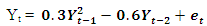
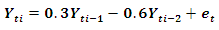
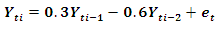
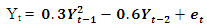
Data is generated from several linear and nonlinear second orders of general classes of autoregressive models as given below: The following codes were written to simulate data from model 1 abovex <- e <- rnorm(50)for (t in 3:50)x[t] <- 0.3*x[t-1]-0.6*x[t-2]+e[t]
 The following codes were written to simulate data from model 2 abovex <- e <- rnorm(50)for (t in 3:150) x[t] <- 0.3*sin(x[t - 1])-0.6*cos(x[t - 2])+ w[t]
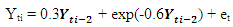
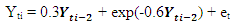
 The following codes were written to simulate data from model 3 abovex <- e <- rnorm(50)for (t in 3:150) x[t] <- 0.3*x[t - 1]+exp(-0.6*x[t - 2]) + e[t]
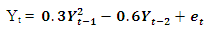
 The following codes were written to simulate data from model 4 abovex<- e <- rnorm(50)for (t in 3:50) x[t] <- 0.3 * (x[t - 1])^2-0.6*x[t - 2] + e[t]
 .
.  Simulation studies were conducted to investigate the performance of autoregressive, self exciting threshold autoregressive, Smooth transition autoregressive models and logistic Smooth transition autoregressive models in predicting h-steps ahead(where h = 5, 10, . . ., 50) from data generated from different general classes of linear and nonlinear autoregressive time series stated above. Effect of sample size was examined on each of the general linear and nonlinear data simulated. Note that in autoregressive modeling, the innovation (error), et process is often specified as independent and identically normally distributed. The normal error assumption implies that the stationary time series is also a normal process; that is, any finite set of time series observations are jointly normal. For example, the pair (Y1,Y2) has a bivariate normal distribution and so does any pair of Y’s; the triple (Y1,Y2,Y3) has a trivariate normal distribution and so does any triple of Y’s, and so forth. Indeed, this is one of the basic assumptions of stationary data. 1000 replications were used to stabilize models estimations at different combinations of sample size (n), steps ahead and models.Selection RuleWe computes MSE and AIC for number of steps ahead, h = 5 10, 15, 20, 25, 30, 35, 40, 45 and 50 for each sample size and model, and select the model that has the minimum criteria values as the best. Note that only second order of autoregressive were considered in each case and situation.
3. Predictive Ability of Fitted Model for Stationary Data
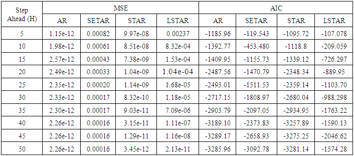
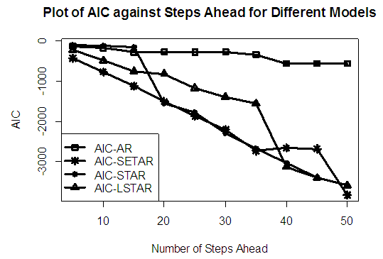
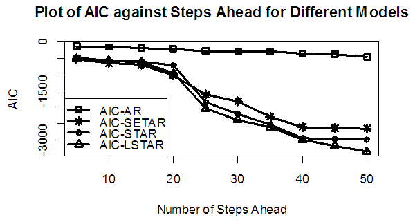
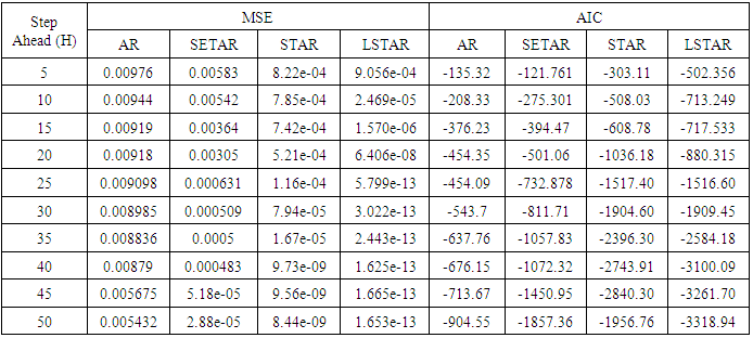
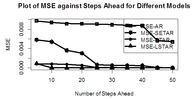
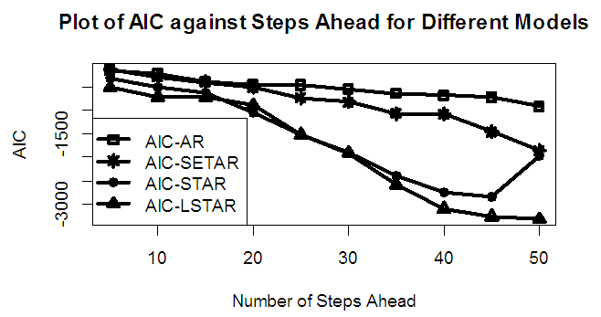
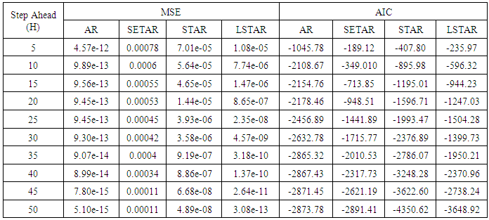
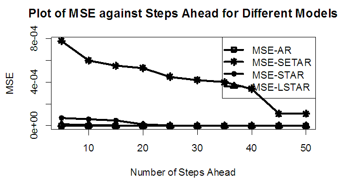
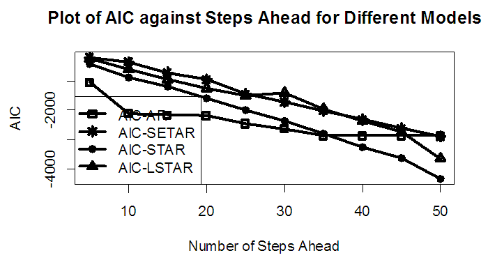
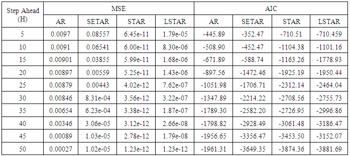
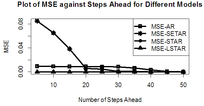
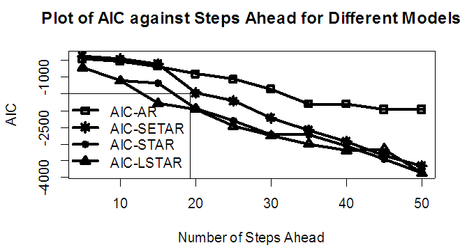
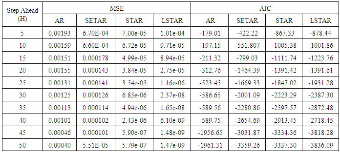
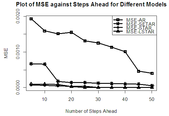
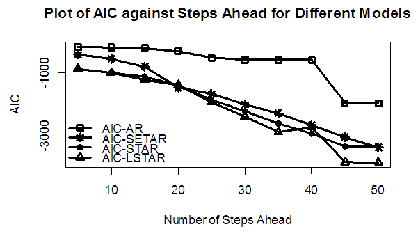
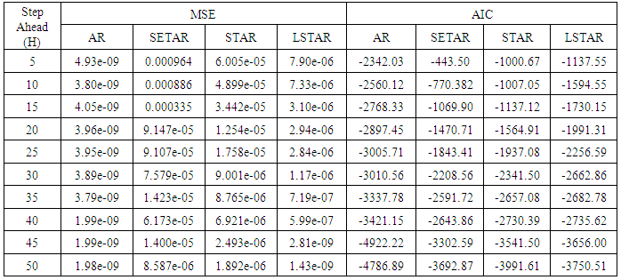
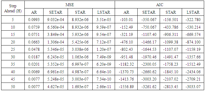
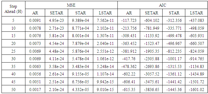
Tables 1-12 shows the comparison of the predictive ability among the four fitted model to model 1, 2, 3 and 4 (linear, trigonometric, exponential and polynomial functions) when sample sizes of 50, 150 and 300 are used in simulation with consideration of stationarity assumptions. The average values of mean square error and AIC of the forecast values of each model at various horizons (H) i.e number of steps ahead and sample sizes were recorded in the tables. The results obtained were plotted on graphs as shown in figures 1a – 12b for more clarity.Table 1. Forecasting Performances of the Fitted Models on the Basis of MSE and AIC With Sample Size of 50 on Model 1(Stationary): AR(2):
 |
| |
|
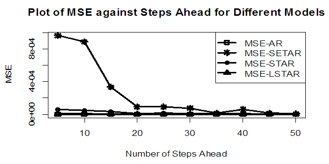
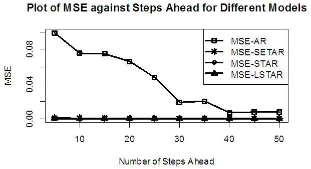
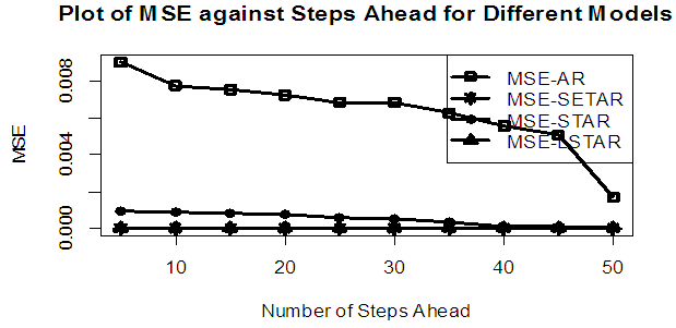
 | Figure 1a. MSE of Forecast Values for the Fitted Models on Model 1 |
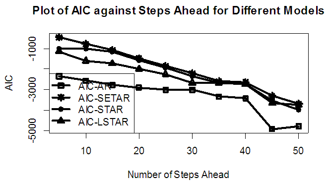
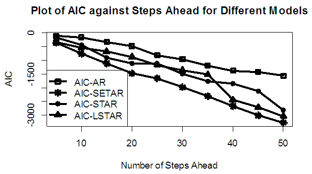
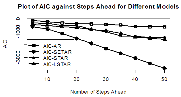
 | Figure 1b. AIC of Forecast Values for the Fitted Models on Model 1 |
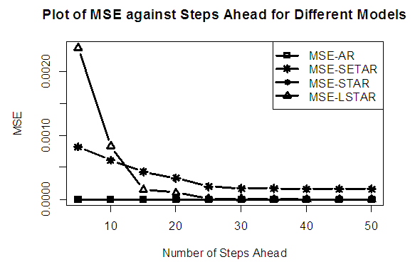
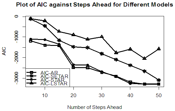
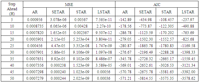
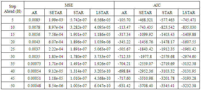
Table 2. Forecasting Performances of the Fitted Models on the Basis of MSE and AIC With Sample Size of 50 for Model 2 (Stationary): TR(2):

 |
| |
|
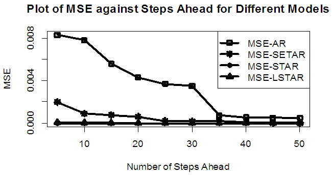
 | Figure 2a. MSE of Forecast Values for the Fitted Models on Model 2 |
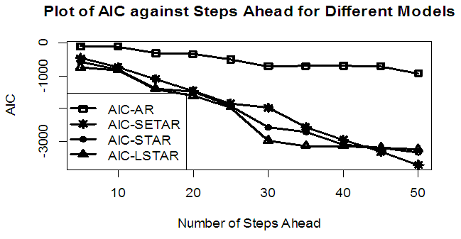
 | Figure 2b. AIC of Forecast Values for the Fitted Models on Model 2 |
Table 3. Forecasting Performances of the Fitted Models on the Basis of MSE and AIC with Sample Size of 50 for Model 3(Stationary): EX(2):
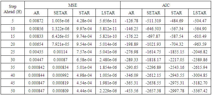 |
| |
|
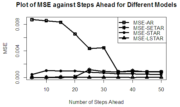 | Figure 3a. MSE of Forecast Values for the Fitted Models on Model 3 |
 | Figure 3b. AIC of Forecast Values for the Fitted Models on Model 3 |
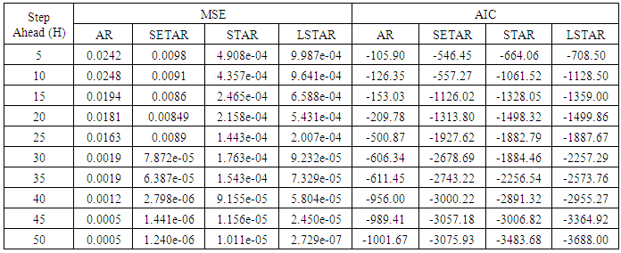
Table 4. Forecasting Performances of the Fitted Models on the Basis of MSE and AIC With Sample Size of 50 for model 4(Stationary): PL(2):
 |
| |
|
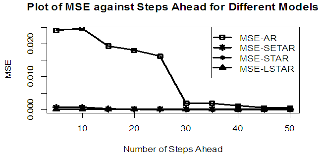
 | Figure 4a. MSE of Forecast Values for the Fitted Models on Model 4 |
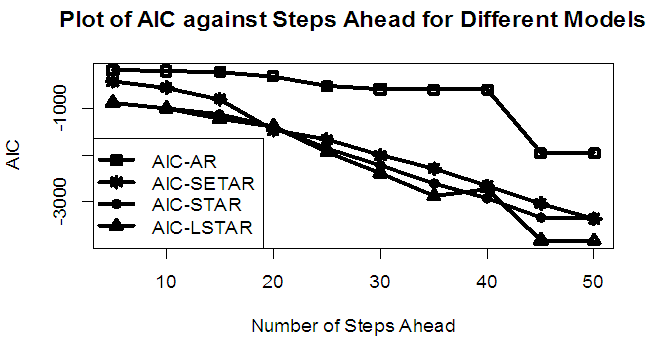
 | Figure 4b. AIC of Forecast Values for the Fitted Models on Model 4 |
Table 5. Forecasting Performances of the Fitted Models on the Basis of MSE and AIC With Sample Size of 150 for model 1 (Stationary): AR(2):
 |
| |
|
 | Figure 5a. MSE of forecast values for the Fitted Models on Model 1 |
 | Figure 5b. AIC of Forecast Values for the Fitted Models on Model 1 |
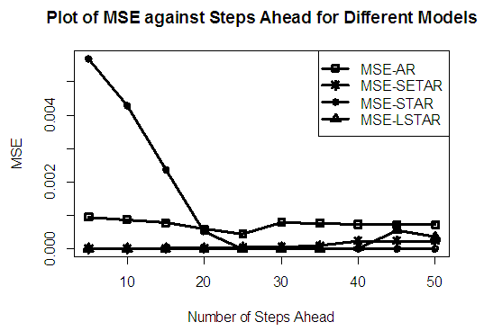
Table 6. Forecasting Performances of the Fitted Models on the Basis of MSE and AIC with Sample Size of 150 for Model 2(Stationary): TR(2):

 |
| |
|
 | Figure 6a. MSE of Forecast Values for the Fitted Models on Model 2 |
 | Figure 6b. AIC of Forecast Values for the Fitted Models on Model 2 |
Table 7. Forecasting Performances of the Fitted Models on the Basis of MSE and AIC with Sample size of 150 for model 3 (Stationary): EX(2):
 |
| |
|
 | Figure 7a. MSE of Forecast Values for the Fitted Models on Model 3 |
 | Figure 7b. AIC of Forecast Values for the Fitted Models on Model 3 |
Table 8. Forecasting Performances of the Fitted Models on the Basis of MSE and AIC with Sample size of 150 for model 4 (Stationary): PL(2):
 |
| |
|
 | Figure 8a. MSE of Forecast Values for the Fitted Models on Model 4 |
 | Figure 8b. AIC of Forecast Values for the Fitted Models on Model 4 |
Table 9. Forecasting Performances of the Fitted Models on the Basis of MSE and AIC With Sample Size of 300 for model 1: AR(2) (Stationary):
 |
| |
|
 | Figure 9a. MSE of Forecast Values for the Fitted Models on Model 1 |
 | Figure 9b. AIC of Forecast Values for the Fitted Models on Model 1 |
Table 10. Forecasting Performances of the Fitted Models on the Basis of MSE and AIC with Sample Size of 300 for Model 2 (Stationary): TR(2):
 |
| |
|
 | Figure 10a. MSE of Forecast Values for the Fitted Models on Model 2 |
 | Figure 10b. AIC of Forecast Values for the Fitted Models on Model 2 |
Table 11. Forecasting Performances of the Fitted Models on the Basis of MSE and AIC with Sample size of 300 for model 3 (Stationary): EX(2):

 |
| |
|
 | Figure 11a. MSE of Forecast Values for the Fitted Models on Model 3 |
 | Figure 11b. AIC of Forecast Values for the Fitted Models on Model 3 |
Table 12. Forecasting Performances of the Fitted Models on the Basis of MSE and AIC with Sample size of 150 for model 4(Stationary): PL(2):
 |
| |
|
 | Figure 12a. MSE of Forecast Values for the Fitted Models on Model 4 |
 | Figure 12b. AIC of Forecast Values for the Fitted Models on Model 4 |
4. Summary of Findings
Tables 1-12 shows the comparison among predictive ability of the four fitted model to model 1, 2, 3 and 4 (linear, trigonometric, exponential and polynomial functions) when sample sizes of 50, 150 and 300 are used in simulation. The average values of MSE and AIC of the forecast values of each model at various horizons (H) i.e number of steps ahead and sample sizes were recorded in tables 1-12. The results obtained were plotted on the graphs as shown in figures 1a – 12b for better understanding.In model 1: Linear FunctionThe best forecast to model 1 is AR based on both MSE and AIC followed by STAR model for the three sample sizes. AR, STAR and LSTAR have equal performance on the basis of MSE when the number of steps ahead increases as shown in figures 1a, 1b, 5a, 5b, 9a and 9b.In model 2: Trigonometric FunctionFrom figures 2a and 2b, using sample size of 50, it was observed that SETAR forecast best to trigonometric function at different horizons based on MSE and AIC followed by LSTAR model. However, the performance of LSTAR model supersede other models as number of steps ahead increases Figure 6a and 6b show that the best forecast to model 2 on the basis of the two criteria of assessment is LSTAR. However, the performance of other three models compete well with LSTAR as number of steps ahead increases on the basis of MSE.Furthermore, in figure 10a and 10b, the best forecast was observed for LSTAR models at different steps ahead followed by STAR except between 45 and 50 horizons where the SETAR model performs better than others. The worst forecast from trigonometric function was observed from linear AR especially at various horizons but its performance improves with increase in number of steps ahead with other models. In model 3: Exponential FunctionFigure 3a and 3b show that LSTAR forecast best to exponential function especially at larger number of steps ahead followed by STAR. However, the performances of the three nonlinear models are similar when sample size increases and the same at smaller sample size. In Figure 7a and 7b, it was observed that LSTAR and STAR models perform almost equally as number of steps ahead increases on the basis of MSE, however the best forecast can be seen clearly to be LSTAR at various horizon from model 2, data simulated from trigonometric function on the basis of the AIC criteria of assessment. From figure 11a and 11b, it can be seen that the SETAR model forecast ahead from exponential function more absolutely well than other models at sample size of 300. However, the performances of the three models increases when sample size increases based on AIC criterion.In model 4: Polynomial FunctionIn figure 4a and 4b, the best forecast was observed for LSTAR models at different steps ahead followed by STAR except between 10 and 20 where STAR model performs better than others. The worst model to fit polynomial function was observed from linear AR especially at larger horizons but their performance improves with increase in number of steps ahead and three nonlinear models converges based on MSE. The results of table 8 plotted in figure 8a and 8b show that the LSTAR model has the best forecast followed by STAR at horizons that are less than 25 and SETAR at above 25 horizons with smallest AIC and MSE criteria. The results in table 12, plotted in fig. 12a and 12b showed that the performance of SETAR and LSTAR are almost the same on the basis of MSE but the SETAR model forecast ahead more absolutely well than other models using sample size of 300 follow by LSTAR. However, the performances of the three models increases when sample size increases based on AIC criterion.
5. Conclusions
The best model to forecast linear autoregressive function is AR. The performance of LSTAR model supersedes other models as number of steps ahead increases in nonlinear time series data except in polynomial function where SETAR model performs better than others. The three nonlinear models SETAR, LSTAR and STAR have closed forecast performances as number of steps ahead and sample sizes increase based on MSE. The predictive ability of the four fitted models increases as sample size and number of steps ahead increase.
References
| [1] | Akaike, H. (1973). “Maximum likelihood identification of Gaussian auto-regressive moving-average models.” Biometrika, 60, 255–266. |
| [2] | Boero, G. and Marrocu, E. (2002), The performance of non-linear exchange rate models: a forecasting comparison, Journal of Forecasting, Vol. 21(7), 513-542. |
| [3] | Boero, G. and Marrocu, E. (2003), The performance of SETAR models: a regime conditional evaluation of point, interval and density forecasts. Working Paper. |
| [4] | Burhnam K.P, and Anderson DR (1998). Model selection and inference: a practical information theoretic approach. New York: Springer. |
| [5] | Clements, M. and Smith, J. (2001), Evaluating forecasts from SETAR models of exchange rates, Journal of International Money and Finance, Vol. 20(1), 133-148. |
| [6] | CHRISTOFFERSEN, P. (1998), “Evaluating interval forecasts”, International Economic Review, 841-862. |
| [7] | Diebold, F. X. and J. A. Nason, 1990, Nonparametric exchange rate prediction, Journal of International Economics, 28, 315-332. |
| [8] | De Gooijer, J. G. and K. Kumar, 1992, Some recent developments in non-linear time series modelling, testing and forecasting, International Journal of Forecasting, 8, 135-156. |
| [9] | Hansen, B. (1996), Inference when a nuisance parameter is not identified under the null hypothesis, Econometrica, Vol. 64(2), 413-430. |
| [10] | Hansen, B. (2001), The new econometrics of structural change: dating breaks in U.S. labor productivity, Journal of Economic Perspectives, Vol. 15(4), 117-128. |
| [11] | Kapetanios, G. and Shin, Y. (2006), Unit root tests in three-regime, Econometrics Journal, Vol. 9(2), 252-278. |
| [12] | Subba Rao, T. and Gabr, M.M. (1980), A Test for Linearity of Stationary Time series. Journal of Time series Analysis 1(1) 145-158. |
| [13] | Wallis, K.F. (2002), “Chi-squared Tests of Interval and Density Forecasts, and the Bank of England’s Fan Charts”, International Journal of Forecasting, forthcoming. |
 Abstract
 Reference
 Full-Text PDF
 Full-text HTML