Oyindamola B. Yusuf1, Linda O. Ugalahi2
1Department of Epidemiology and Medical Statistics, University of Ibadan, Oyo State, Nigeria (Senior lecturer in Medical Statistics)
2Department of Epidemiology and Medical Statistics, University of Ibadan, Oyo State, Nigeria (Postgraduate trainee in Medical statistics)
Correspondence to: Oyindamola B. Yusuf, Department of Epidemiology and Medical Statistics, University of Ibadan, Oyo State, Nigeria (Senior lecturer in Medical Statistics).
| Email: |  |
Copyright © 2015 Scientific & Academic Publishing. All Rights Reserved.
Abstract
The number of visits to an antenatal care (ANC) facility is a count variable and it is often modeled by the Poisson regression, however it is sometimes erroneously used in situations where over dispersion (i.e. the variance of the response variable exceeds the mean) occurs. Negative Binomial and Generalised Poisson regression models are alternative models for estimating regression parameters in the presence of over dispersion. This analysis compared Poisson, Negative Binomial and Generalized Poisson regression models to determine the best statistical model which describes the utilisation of ANC visits. A nationally representative sample of women within reproductive age (15-49 years) within households in communities was obtained from the 2013 National Demographic and Health Survey (NDHS) dataset. The number of ANC visits was the outcome variable and other explanatory variables include age, region, employment status, wealth index, husband’s/partner’s employment status, husband’s/partner’s educational level, place of residence and place of ANC. The Poisson, Negative Binomial and Generalized Poisson regression models where fitted to the data at 5% significance level. The best model was selected based on the values of -2logL, AIC and BIC selection test/criteria. Of the three regression models, Generalized Poisson regression had the least -2logL, AIC and BIC. Age (35-49 years) (IRR = 1.142, 95% CI: 1.053, 1.240) and rural place of residence (IRR=0.910, 95% CI: 0.874, 0.947) were some of the significant predictors of the number of ANC visits. In the presence of over dispersion, Generalised Poisson Regression was the best regression model in identifying factors associated with the number of antenatal care visits.
Keywords:
Over dispersion, Model comparison, Number of ANC visits
Cite this paper: Oyindamola B. Yusuf, Linda O. Ugalahi, On the Performance of the Poisson, Negative Binomial and Generalized Poisson Regression Models in the Prediction of Antenatal Care Visits in Nigeria, American Journal of Mathematics and Statistics, Vol. 5 No. 3, 2015, pp. 128-136. doi: 10.5923/j.ajms.20150503.04.
1. Introduction
Maternal mortality is an important pointer to maternal health and well-being of a country. The health/ survival of a child and the welfare of a family is affected by maternal mortality and morbidity [1]. Maternal mortality is defined by the World Health Organization as “the death of a woman while pregnant or within 42 days of a termination of a pregnancy irrespective of the duration and the site of the pregnancy, from any cause related or aggravated by the pregnancy or its management but not from accidental and incidental causes” [2].The Millennium Development Goal 5 (MDG 5) focuses on improving maternal health and reducing maternal mortality by 75 percent by 2015 from what it was in 1990. Subsequently in 2006, the introduction of a second target was included which is to achieve universal access to health facilities by reproductive age women (15-49yrs) by 2015 [1].In 2008, the estimated number of women getting prenatal care was about 58 percent in Nigeria according to the World Bank, (2013) [3]. These are the women who attended at least one visit connected to or during pregnancy and were attended to by a skilled health worker. The women in urban areas utilized ANC visits more compared to those in rural areas [4].Utilization of ANC facility is measured by the number of visits a woman makes to such a facility. The number of ANC visits is a count variable which takes non negative integer values. Poisson regression is widely used to model count outcomes however it is sometimes erroneously used in situations where over dispersion occurs i.e. variance of the response variable exceeds the mean. It is inappropriate to use Poisson regression as it underestimates the standard error and exaggerates the significance of regression parameters [5] [6]. Due to the heterogeneous nature of data, over dispersion usually occur in such count outcome variables. There is more variability around the model’s fitted values than is consistent with a Poisson formulation i.e. the mean does not equal the variance; over dispersion [7]. To correct this problem, the negative binomial Regression and generalised Poisson regression which are more special cases of the generalised linear model were used to model number of ANC visits.In this analysis, we applied the Poisson, Negative Binomial and Generalised Poisson regression models to the National Demographic and Health Survey (NDHS 2013) dataset to determine which model best fits the nature of the outcome variable; number of visits to an antenatal facility. It also suggests the Negative Binomial and Generalised Poisson regression models as alternative models for handling over dispersion. Furthermore, these models were compared to ascertain which model best describes over dispersion. The objective of this study was to determine the best statistical model that describes the utilization of antenatal care visits.
2. Methodology
This study is a secondary analysis of the National Demographic and Health Survey (NDHS) dataset, a nationally representative survey conducted in 2013. Administratively, Nigeria has 36 states and Federal Capital Territory (FCT). These were divided into local government areas (LGA) and each LGA was further divided into smaller localities. The 36 states were regrouped by geopolitical location into six zones and using the 2006 Population census implementation, each locality was subdivided into Enumeration Areas (EAs). A complete list of the EAs served as the sample frame of the survey. The sampling technique for the 2013 NDHS was a stratified sample, selected at random in three stages from the sampling frame. At the first stage; each state was stratified into urban and rural areas; this resulted in a list of localities. Second stage; one enumeration area was randomly selected from a selected locality with equal probability selection, the resulting list of households served as sampling frame for the selection of households in the third stage. At the third stage; 45 households were selected in every urban and rural cluster through equal probability systematic sampling using the household listing. More details can be obtained from the NDHS report, 2013 [8].Simple summary statistics (percentage for categorical variables or mean for continuous variables) for all independent variables was also performed. Sample mean and sample variance of the dependent variable (number of antenatal care visits) was calculated to check for the presence of over dispersion or under dispersion. Pearson chi-square and Deviance was utilized to evaluate the presence of over dispersion. These ascertained whether the data followed a standard Poisson, Negative Binomial or the Generalised Poisson regression models. The Poisson, Negative Binomial and Generalised Poisson regression parameters were estimated, 95% confidence intervals and incidence rate ratios (IRR) were reported. SPSS version 20 and STATA version 12 were used for analysis.
2.1. The Poisson Regression
Poisson regression is used in situations where the dependent variable is a count variable; the counts are positive integers and has a mean greater than zero. A Poisson distribution is derived as a limiting form of binomial distribution when the number of trials becomes large and the probability of success is small. Poisson regression model expresses the logarithm outcome rate as a linear function of a set of predictors. It makes an important assumption that; for a sample of observations, the mean and the variance of the distribution are equal.A random variable Z is said to have a Poisson distribution with parameter θ if it takes integer values; 0, 1, 2 …∞.The probability distribution is represented as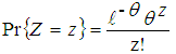 | (2.1) |
With mean and variance represented as;E(Z) = θ and var(Z) = θ respectively.Writing the parameter θ as a log linear model: | (2.2) |
The Poisson regression which was fitted to the number of visits made to antenatal care facility, θ was expressed for the ten independent variables as shown below, where the explanatory variables were: (X1 = Age, X2 = Region, X3 = Residence, X4 = Educational Level, X5 = Religion, X6 = wealth index, X7 = occupation, X8 = place of antenatal, X9 = husband’s/partner’s educational level, X10 = husband’s/ partner’s occupation). | (2.3) |
The parameter β which represents the expected change in the logarithm of the mean per unit change in the predictor Xi can be estimated by the maximum likelihood method.
2.2. The Negative Binomial Regression
Under the Poisson regression the mean θi, is assumed to be homogenous within the classes, however by defining a specific distribution for θi, the classes become heterogeneous. Negative binomial regression model is a more generalised model than the Poisson regression. Making the assumption that the mean θi, follows a gamma distribution with mean E(θi) = µi and variance Var (θi) = µi vi-1. Consider the Poisson distribution Zi |θi with a conditional mean E(Zi |θi) = θi,; the marginal distribution can be shown to follow a Negative Binomial distribution [7].The probability density function of a negative binomial distribution is represented as: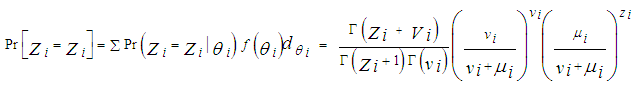 | (2.4) |
Where;Mean is E(Zi) = µi and variance is var(Zi) = µi + µi2vi-1,Vi is the dispersion parameter.The maximum log likelihood function of the distribution is expressed as;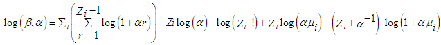 | (2.5) |
The parameters (β, α), can be estimated by partial differentiation of the maximum log likelihood function with respect to β and α.The negative binomial regression does not make the assumption of equality of the mean and variance but it corrects for over dispersion that arises when the variance is greater than the conditional mean.
2.3. The Generalised Poisson Regression
The Generalised Poisson regression model adjusts for both under dispersion and over dispersion properties in a dataset. For the dependent variable; number of visits to antenatal care, represented by Zi, the probability distribution function of a generalised Poisson distribution is given as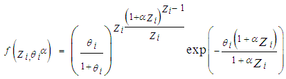 | (2.6) |
Where; z = 0, 1, 2 …∞The standard Poisson regression model is a special form of the generalised Poisson regression model, when α is zero, the probability function of the generalised Poisson random variable reduces to the Poisson probability function. The positive value of α in the equation above indicates over dispersion while a negative value of α indicates under dispersion property of the distribution. The mean of the dependent variable is related to the independent variables through the link function; θi = (xiβ), which is a simple linear model. This model has the disadvantage of θi assuming any real value but a Poisson mean assume only count non negative values. To correct this problem the logarithm of the linear model is used; this gives a link log function:Log(θi)= (xiβ). Taking the exponential of the model we have; θi = exp(xi,β). In the link function, xi is (k-1) dimensional vector of explanatory variables and β is a k dimensional vector of regression parameters and α is a dispersion parameter. The mean and variance of Zi are given by; E(Zi |Xi) = θi, and V(Zi |Xi) = θi(1 + αθi)2 respectively [7] [5].In the generalised Poisson regression model, the parameters (β, α) can be estimated by taking the derivatives of the log likelihood function of the model; this means partial differentiation with respect to β and α of the logarithm function of equation (2.7) below;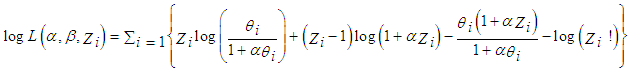 | (2.7) |
2.4. Model Selection
Model selection was used to determine the best statistical model which best approximates reality given the set of data and also minimize loss of information. The following goodness of fit tests were utilized in this analysis for model selection.
2.4.1. Chi-square -2log Likelihood Statistic
The maximized likelihood, L, for a given model is the value of the likelihood function when the parameters are substituted with their maximum likelihood estimates and the statistic -2logL was used to compare models. It is useful for comparing models fitted to the same set of data as the value of L depends on the number of observations in the data and -2logL is a measure of agreement between the model and the data. The larger the maximum likelihood the better the agreement between the model and observed data, but the smaller the value of -2logL the better the model.
2.4.2. Akaike Information Criterion
This method of model selection is based on a relationship between maximum likelihood estimation and Kullback-Leibler information. This information criterion was developed by Akaike. It is derived under the assumption that the operating models belong to the approximating family.AIC = -2log L(θ) + 2KWhere L(θ) is the maximized likelihood function and K is the number of estimated parameters included in the model (number of variables plus the intercept). The log likelihood of the model of the data is the overall fit of the model. The smaller value of the log likelihood indicates a worse fit model. However after comparing different models the model with the minimum AIC value is the best model.In AIC the compromise occurs between maximized log likelihood -2 logL(θ); which is the lack of fit component and k, the number of free parameters estimated within the model which is a measure of the compensation for the bias in the lack of fit when maximum likelihood estimators are used. The term 2k is the penalty term, the reason for using the penalty term is to prevent over fitting [9].AIC uses the log likelihood which is the probability of obtaining the chosen data under the given model; hence it makes sense to choose a model that makes the probability as large as possible. The logarithm does not affect the value but the negative sign does, it means minimizing the value of the statistics.
2.4.3. Algorithm for AIC Cross Validation
The following are the algorithm used for the AIC cross validation:1 Assess AIC for all models.2 Identify the model with the smallest AIC value denoted by AICmin. This is the best model.3 To further compare the models, the AIC difference will be calculated for each model; Di = AICi - AICmin4 Compute the relative likelihood,  for each model5 Compute Akaike weights wi for each model, these are normalized relative likelihoods
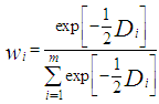 These weights can be interpreted as probabilities; the probability that the given model is the best model.
2.4.4. Bayesian Information Criterion (BIC)
BIC is similar to AIC; the difference is in the second term which depends on the sample size n. BIC = -2log (L) + p log (n)Where L denotes the log likelihood, p the number of parameters and n the number of rating classes or number of observations utilized in the model, the smaller the BIC, the better the model. The derivation of BIC assumes equal priors on each model and uninformative priors on the parameters, given each model [10].The goal of BIC is to find the best model for prediction using highest posterior probability while the goal of AIC is to identify the model that most plausibly generated the data. Both AIC and BIC can be used whether the models are nested or not. Information criterion supply information on the strength of evidence for each model, it does not make use of a significance level rather it is based on maximum likelihood. It has a high potential of selecting the best model as it is independent of the order in which the models are computed. In this study all selection models were utilized, this was to ensure agreement between the three model selection methods in order to select the best model.
3. Results
3.1. Poisson Regression Results
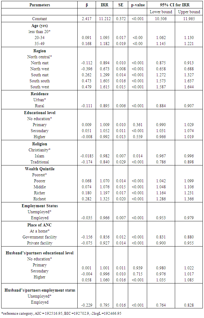
Table 1 shows the regression parameters for Poisson regression. The deviance for the model was about 11.547 times larger than the degree of freedom which indicated the possible existence of over dispersion. Table 1. Parameter estimates for Poisson regression
 |
| |
|
The number of ANC visits was higher by approximately 9.5% among respondents aged 20-34 years compared to respondents aged less than 20 years (IRR= 1.095, 95% CI: 1.062, 1.130). Number of ANC visits among respondents from the south east, was higher by 29.9% (IRR=1.299, 95% CI: 1.272, 1.327), compared to number of ANC visits by respondents in the north central zone. However respondents from the north east and north west had lower number of ANC visits by approximately 10.6% (IRR=0.894, 95% CI: 0.875, 0.913) and 32.7% (IRR=0.673, 95% CI: 0.658, 0.688) respectively compared to respondents from north central. Respondents in rural residence had a 10.5% decrease (IRR=0.895, 95% CI: 0.884, 0.907) in number of ANC visits compared to respondents in urban residence. The number of ANC visits increased by 5.2% among women with secondary education compared to women with no education (IRR=1.052, 95% CI: 1.031, 1.074). Respondents in the richest wealth quintile had a 32.5% increase in number of ANC visits compared to respondents in the poorest wealth quintile (IRR=1.325, 95% CI: 1.286, 1.366).
3.2. Negative Binomial Regression Results
Table 2 shows the regression parameters for Negative Binomial regression, the ratio of deviance to degree of freedom for the model is about 0.70 (approximately 1), this indicates an adjustment for over dispersion. Alpha of the model had a value significantly greater than zero (alpha=0.653, 95% CI = 0.637, 0.671), this showed that the data was better modelled by negative binomial regression due to the presence of over dispersion. The estimates of the standard error were slightly larger than those of the Poisson regression.Table 2. Parameter estimates for Negative Binomial Regression
 |
| |
|
The number of ANC visits was higher by approximately 8.2% among respondents aged 20-34 years compared to respondents aged less than 20 years (IRR= 1.082, 95% CI: 1.000, 1.170). The number of ANC visits in the different geopolitical zones increased by 32% for south east (IRR=1.324, 95% CI: 1.244, 1.410) compared to the north central zone.Respondents in rural areas had a 10.5% decrease (IRR=0.895, 95% CI: 0.884, 0.907) in the number of ANC visits compared to respondents in urban areas. Respondents in the richest wealth quintile had a 27% increase in the number of ANC visits compared to respondents in the poorest wealth quintile (IRR=1.276, 95% CI: 1.178, 1.381). Respondents whose husbands/partners had higher education had a 7.3% increase in the number of ANC visits compared to respondents whose husband/partner had no education (IRR=1.073, 95% CI: 1.007, 1.144).
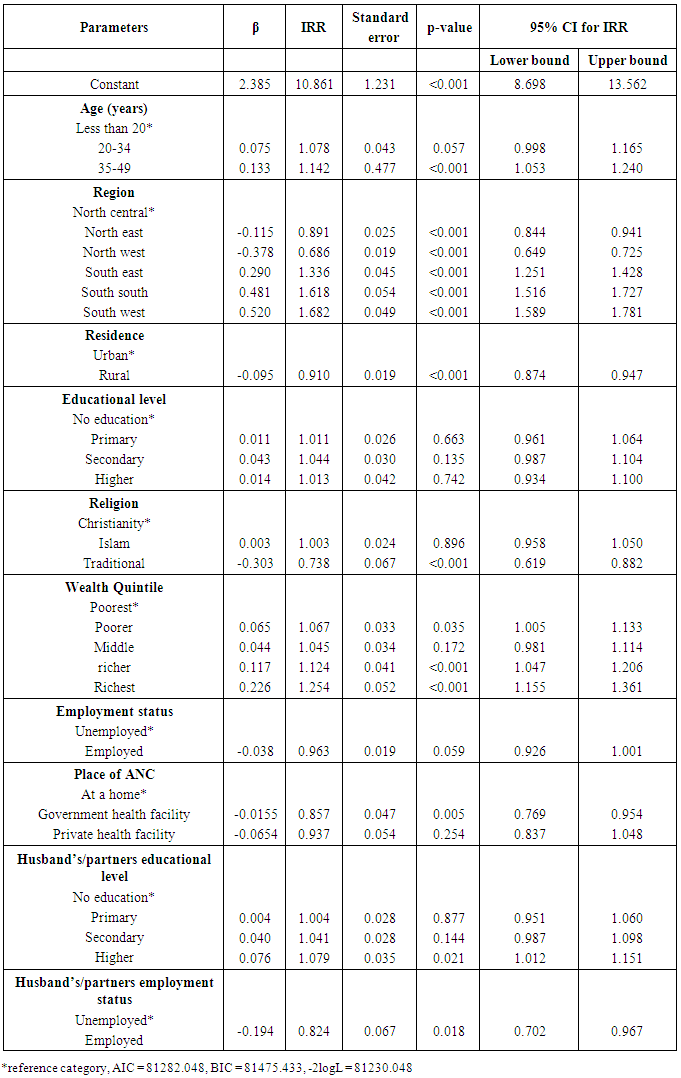
3.3. Generalised Poisson Regression Results
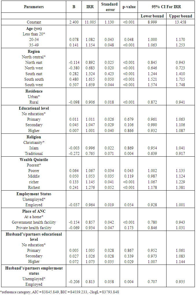
Table 3 shows the regression parameters for Generalised Poisson regression. The positive value of phi (phi=0.182; 95% CI: 0178, 0.186) from the model indicated an adjustment for Poisson over dispersion. The estimates of the standard error were similar to those of the Negative Binomial regression, although slightly higher. Table 3. Parameter estimates for Generalised Poisson regression
 |
| |
|
The number of ANC visits was higher by approximately 14% among respondents aged 35-49 years compared to respondents aged less than 20 years (IRR = 1.142, 95% CI: 1.053, 1.240). The number of ANC visits among respondents increased by 33.6% for south east (IRR = 1.336, 95% CI: 1.251, 1.428), compared to respondents in the north central zone. Respondents in rural areas had about 9% decrease (IRR = 0.910, 95% CI: 0.874, 0.947) in the number of ANC visits compared to respondents in urban areas. Respondents in the richest wealth quintile had a 25% increase in the number of ANC visits compared to respondents in the poorest wealth quintile (IRR = 1.254, 95% CI: 1.155, 1.361). Respondents whose husband/partner had higher education had a 7.9% increase in the number of ANC visits compared to respondents whose husbands/partners had no education (IRR=1.079, 95% CI: 1.012, 1.151).
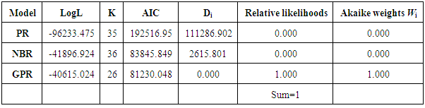
3.4. AIC Cross Validation
Table 4 shows the comparison of the three models PR, NBR and GPR utilising the difference (Di) between the models and the model with the least value, hence the relative likelihood were computed, this led to Akaike weights computation. Using this cross validation of AIC, GPR model would be ranked best model 100% of the time when comparing these three models i.e. PR, NBR and GPR.Table 4. Model comparison using AIC cross validation algorithm
 |
| |
|
4. Discussion
The standard errors from Poisson regression are smaller than those of Negative Binomial regression, the relatively larger values of NBR standard errors led to some insignificant regression parameters. Similarly larger standard errors of the parameters in the GPR model led to more insignificant regression parameters. The large standard error in NBR and GPR shows that in the presence of over dispersion, the Poisson regression overstates the significance of the regression parameter and the significance of the evaluation factors. This is compatible with findings from other studies [11] [5] [7] [12]. Generalised Poisson regression was the best model selected. This was inferred from the values of the model selection test/criteria utilized. These are -2logL, AIC and BIC. All these criteria established the GPR as the best model because it had the smallest value of all three selection criteria. The cross validation of AIC agrees with the selection of GPR as the best model for count data in the presence of over dispersion.This study demonstrated that GPR model is the best model to determine the factors that predict the number of antenatal care visits to a health care facility, when there is an indication of the presence of over dispersion. It is recommended that objective criteria should be used to select appropriate statistical models for analysing count data in the presence of over dispersion.
References
| [1] | S. H. Adamu, Utilisation of Maternal Health Care Services in Nigeria: An Analysis of Regional Differences in the Patterns and Determinants of Maternal Health Care Use, 2011. Available at: http://mph/MPHQuantitativeDisertation. |
| [2] | WHO. Making pregnancy safer: the critical role of the skilled attendant. A joint statement by WHO, ICM and FIGO. Geneva, Switzerland WHO. 2000, Available at: http://whqlibdoc.who.int/publications/2004/9241591692.pdf. |
| [3] | World Bank. Pregnant women receiving prenatal care (%). The World Bank Data. Available at: http://data.worldbank.org/indicator. |
| [4] | B. I. Babalola, T. O. Adeyoju, and A. Makumi, Determinants Of Urban-Rural Differentials in Antenatal care utilisation in Nigeria, presented at Population Association of America New Orleans, April 2013. |
| [5] | N. Ismail and A.A. Jemain, “Handling Overdispersion with Negative Binomial and Generalized Poisson Regression Models,” Casualty Actuarial Society Forum Winter, 2007 pp. 103–158. |
| [6] | G. Sileshi, “Selecting the right statistical model for analysis of insect count data by using information theoretic measures”. Bulletin of Entomological Research, 2006 vol. 96 pp.479-488. |
| [7] | F. Sadia, Performance of Generalized Poisson Regression Model and Negative Binomial Regression Model in case of Over-dispersion Count Data,2013, pp. 558–563. |
| [8] | National Population Commission. Nigeria Demographic and Health Survey: Preliminary Report, 2012. Available from: http://dhsprogram.com/pubs/pdf/PR41/PR41.pdf |
| [9] | H. Bozdogan, “Akaike’s Information Criterion and Recent Developments in Information Complexity,” Journal of Mathematical Psychology, 2000 vol. 44 pp. 62–91. |
| [10] | W. Zucchini, “An Introduction to Model Selection.” Journal of Mathematical Psychology, 2000 vol. 44 pp. 41–61. |
| [11] | B.E.L. Piza, Using Poisson and Negative Binomial Regression Models to Measure the Influence of Risk on Crime Incident Counts. 2012 Available at: http://rutgerscps.weebly.com/uploads/2/7/3/7/27370595/countregressionmodels.pdf. |
| [12] | M.M. Islam, M. Alam, M. Tariquzaman, M.A. Kabir, R. Pervin, M. Begum, et al. Predictors of the number of under-five malnourished children in Bangladesh: application of the generalized poisson regression model. BMC Public Health, 2013, vol. 13 pp. 11. Available at: http://www.pubmedcentral.nih.gov. |
 Abstract
 Reference
 Full-Text PDF
 Full-text HTML