1. Introduction

Gini’s mean difference (GMD) depends on all pairwise distances rather than square of the data and has been used as an alternative to the standard deviation in many fields. The Gini’s coefficient is a most used measure of inequality; see, [1], [2] and [3]. It is known that the GMD has asymptotic relative efficiency of 98% at the normal distribution and more efficient than standard deviation if the normal distribution is contaminated by a small fraction; see, [8], [5] and [6]. It may also offer certain pedagogical advantages; see, [7]. For extensive discussion and comparisons; see [6] and [8] and the references therein.

The population GMD is defined as

It can be estimated from the sample using many formulas such as

See, for example, [8].

A random variable has a normal distribution with location parameter and scale if its probability density function is

The normal distribution has

Therefore,

This will be used later in simulation studies.

A randomized complete block design is a restricted randomization design in which the experimental units are first sorted into homogeneous rows, called blocks, and the groups (treatments) are then assigned at random within the blocks; see, [9]. The model for a randomized complete block design containing the comparison of no interaction effects, when both the block and treatment effects are fixed and there are B blocks (BL) and G groups (TR), is as

is a constant, are constants for the block (row) effects, are constants for the group (column) effects and are independent normally distributed with mean 0.

Analysis of Gini’s mean difference (ANOMD) for a randomized block design is derived where the total sum of difference (TSD) is partition into exact block sum of difference (BLSD), exact treatment sum of difference (TRSD) and within sum of difference (WSD). The exact partitions are derived by getting rid of the absolute function from Gini’s mean difference (GMD) by using the idea of redefined the GMD as a weighted average of the data with sum of weights zero. TSD does not depend on any fixed location and this is logic where TSD is the total of all pairwise distances while BLSD, TRSD and WSD are depending on any fixed location. This exact partition is used for comparison of several mean and median values. A simulation study is conducted to obtain the critical values for the ratios of mean BLSD to mean WSD and mean TRSD to mean WSD based on normal distribution. Two ANOMD graphs are proposed based on BLSD and WSD. However, two tests for means and medians are proposed under the assumption of normal distribution. The effect size measures are suggested under ANOMD. These measures are shown that the percentage of explained variation based on ANOMD is more than the percentage of explained variation based on ANOVA.

Representation of GMD as a weighted average is presented in Section 2. The partitions of TSD into exact BLSD and exact WSD are derived in Section 3. The critical values for ratios are obtained in Section 4. Two graphs are proposed in Section 5. ANOMD tests for mean and median with effect sizes are studied in Section 6. Section 7 is devoted to conclusion.

2. Representation of GMD as a Weighted Average

Let be a random sample from a continuous distribution with, density function , quantile function , , cumulative distribution function and the order statistics. There is a relationship between the second L-moment and GMD where the second L-moment is a half GMD, therefore

Hence,

From [9] and [10] this can be estimated as

3. Exact GMD Partitions about Mean and Median

Assume there are G different groups (treatments) with individuals in each group , with block and . Let is the total deviation , is the deviation of group mean around total mean, is the deviation of block mean around total mean and is the error or within.

The sample GMD is

This can be rewritten without order and taking the rank of y as

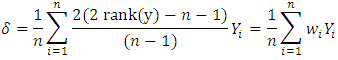This is a weighted average form where

Note that,

Therefore, the total sum of differences (TSD) is considered as

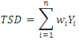This is the most important equation to obtain the exact analysis of total differences as follows.

Theorem 1

In a randomized complete block design the total sum of differences about mean is partitions as

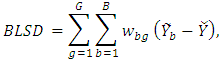
where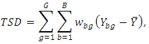

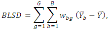
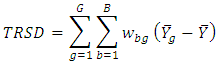
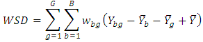
and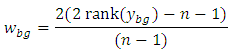

Proof:

Where , the total sum of differences is

By adding and subtracting and taking the summation over both then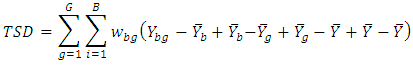

Therefore,

Theorem 2

In a randomized complete block design the total sum of differences about median is partitions as

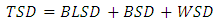where

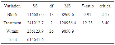
Proof: same as mean.

Comparison with ANOVA

The analysis of variance (ANOVA) for a randomized complete block design is

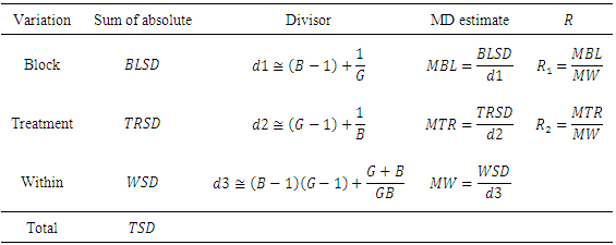
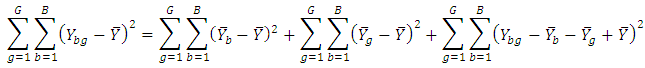See; for example, [12].

The analysis of Gini’s mean difference (ANOMD) for a randomized complete block design is

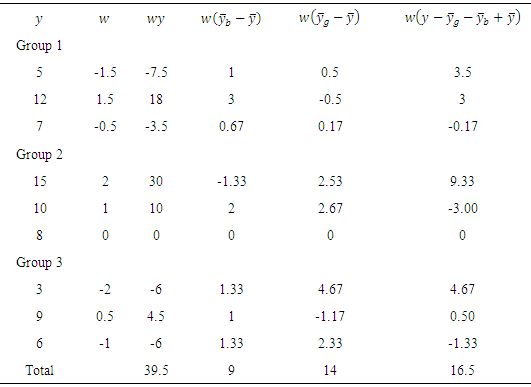
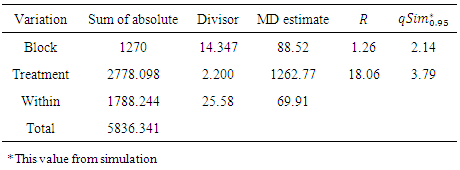
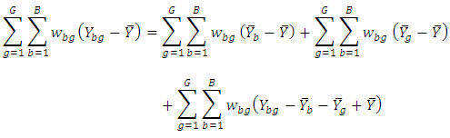Note that:

1. ANOMD replaces the square in ANOVA by weights and that ensures stability in statistical inferences.

2. ANOMD can be extended to any measure of location (median) easily where TSD does not depend on any fixed location and this is logic where TSD is the sum of all pairwise distances.

Illustrative example

To have an idea on how the method work. Table 1 shows TSD partition for a hypothetical data. Note that, and the total is 39.5 that gives exact partitions.

Table 1. TSD partition into BLSD, TRSD and WSD for a hypothetical data

3.1. Divisors and ANOMD Tables

ANOMD is introduced and used to test for population means and medians under the following assumptions.

1. The observations are random and independent samples from the populations.

2. The distributions of the populations from which the samples are selected are normal.

3. The of the distributions in the populations are equals.

A simulation study is conducted to compute the suitable divisors for scaled BLSD, TRSD and WSD using the following steps:

1. For selected design simulate data from normal distribution using a very large number N.

2. Compute .

3. Compute the average for each one.

Table 2. Simulated averages for       with different values of G and B from normal distribution and the number of replications is 10000

From the simulation results in Table 2, the proposed ANOMD table about mean is summarized in Table 3.

Table 3. Summary of ANOMD table for mean

Also, from the simulation results in Table 2, the proposed ANOMD table about median is summarized in Table 4.

Table 4. Summary of ANOMD table for median

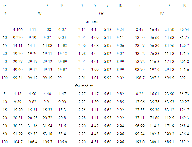
4. Simulation Approach for Critical Values

The following steps are used to obtain the critical values:

1. For any given design simulate data from normal distribution using large number N.

2. Compute R for each N.

3. Use quantile function in software R to obtain the required quantile for R.

Table 5. Simulated critical values for R1 and R2 using normal distribution for different B and G and the number of replications is 10000

Table 6. Simulated critical values for R3 and R4 using normal distribution for different B and G and the number of replications is 10000

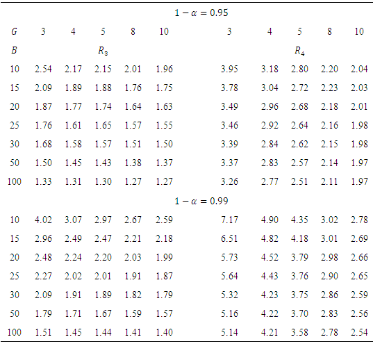
Tables 5 and 6 give the simulated critical values for based on normal distribution for different values of B and G.

5. Graphic Presentation

5.1. ANOMD General Plot

This plot is for all groups to detect shifts in means or medians. The contains the index of the groups and the contains the heights for the sum of , and for each group. Note that mean is used as an example. Separate curves are drawn for sum of . The points on each curve are connected by lines. This graph should reflect the heights, shifts, and patterns among all groups.

5.2. ANOMAD Individual Plot

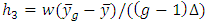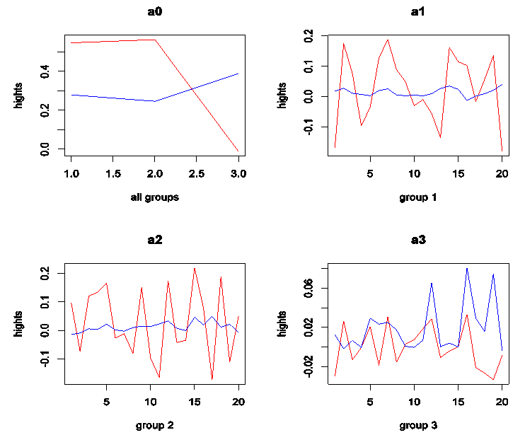
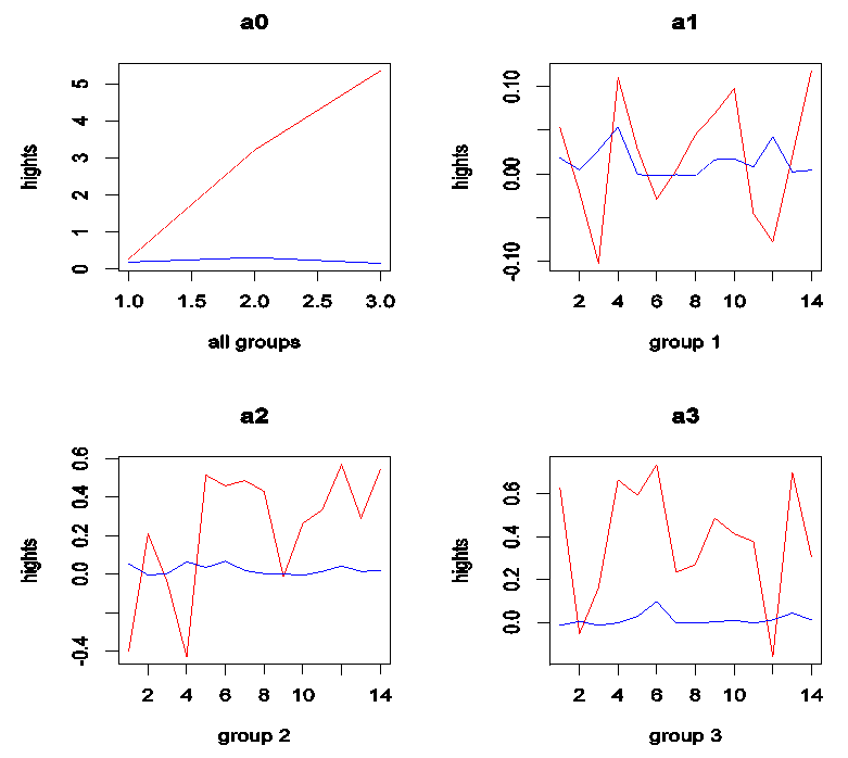
This plot is for each group to detect shifts inside the group. The contains the index of the data for each group and the contains the heights, and for each value. Separate curves are drawn . The points on each curve are connected by lines. This graph should reflect the heights, shifts and patterns in each group.Figures 1, 2 and 3 show that:

1. When means or medians are equals the two lines will be near from each other and most likely that there will be interference among them or the treatment line may be down the within line; see, Figures 1 and 2 a0. In this case it will not be clear pattern in each group and the heights will be almost the same for on each group; see, Figures 1 and 2 a1, a2 and a3. This may be indicating a strong evidence for no shifts in means or medians.

2. When mean(s) or median(s) are not equals the treatment line will start to go up until it may be separated from the within line; see, Figure 3 a0. In this case it will be clear pattern in group(s) with clear different gaps or heights; see, Figure 3 a1, a2 and a3. It is clear that the second group has a different pattern from others. This may give a strong evidence for shift (s) in mean(s) or median(s).

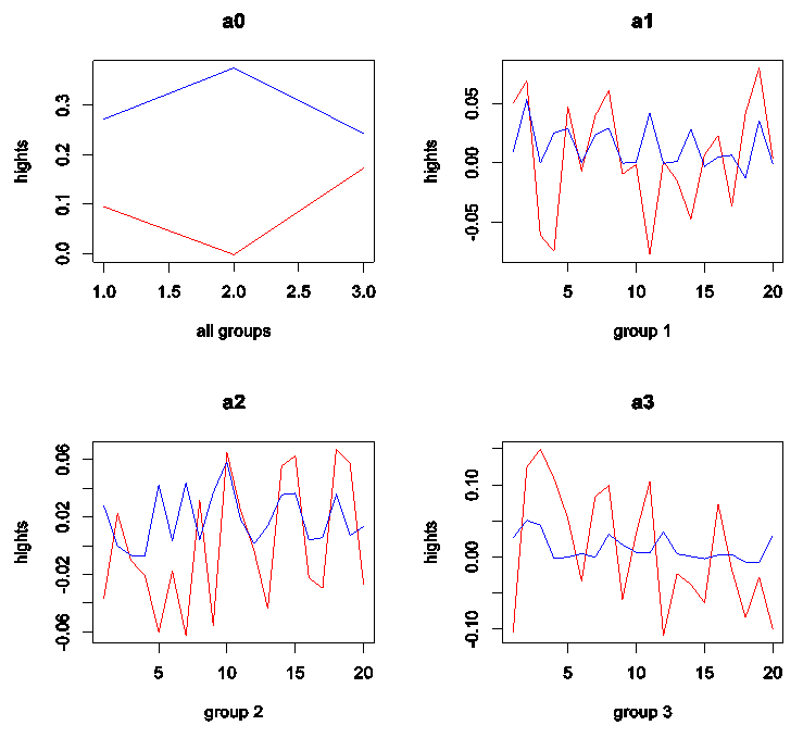Figure 1. ANOMD plot for simulated data from N(10,1): (a0) all groups and (a1), (a2) and (a3) for each group and G = 3, n = 60. Red line is treatment and blue line is within

Figure 2. ANOMD plot for simulated four groups N(10,1) and one group N(10.5,1): (a0) all groups and (a1), (a2), and (a3) for each group and G = 3, n = 20. Red line is treatment and blue line is within

Figure 3. ANOMD plot for simulated four groups N(10,1) and one group N(12,1): (a0) all groups and (a1), (a2), and (a3) for each group and G = 3, n = 60 . Red line is treatment and blue line is within

6. Test for Mean and Median

For mean the null hypothesis is that

Blocks

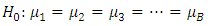Treatments

For median the null hypothesis is that

Blocks

Treatments

Fresh & fun is a food chain with three outlets; see, [12]. The owner is interested in testing the average service quality at the three outlets. Fourteen people are selected and they asked to eat at each of the three outlets. The order of visits to the three outlets was randomized, but each customer visited each outlet one time. After each visit, each customer rated the service on a scale of 1 to 100. The data is given in Table 7.

To test for the assumption of normal distribution, the function shapiro.test() in R-software is used. Table 7 gives the sample data with means, medians, MD and Shapiro-wilk test for normal distribution. The results for the three groups are given in Table 7 where more than 0.01, 0.05 and 0.10, therefore, the assumption of normal cannot be rejected. Because the maximum MD to minimum MD is 1.4, the assumption of homogeneity of may not be rejected.

Table 7. Service quality score for three outlets and normal test

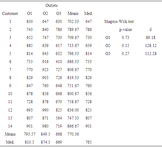
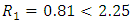From Table 8, since the null hypothesis could not be reject, .i.e., blocking is not effective while , therefore, the outlets are different in averages.

Table 8. ANOMD for testing means for quality service

Figure 4 shows that

1. Most of the points of treatment line are above the within line with a big gap. This might give a visual evidence of shift in average; see, Figure 4 a0.

2. The first group is stable while the second and third groups have big shifts. The second group has pattern near from third group but the gaps or heights are much more than the other groups. This may indicate that the third group is different from others; see, Figure 4 a1, a2 and a3.

Figure 4. ANOMD plots for the service quality data for three outlets

Table 9 shows that the block is not significance while the treatment is significance for testing medians.

Table 9. ANOMD for testing medians for quality service

The ANOVA table for the above data is given in Table 10.

Table 10. ANOVA for quality service data

6.1. Effect Sizes

Effect sizes (ES) provide another measure of the magnitude of the difference expressed in standard variation units in the original measurement. Thus, with the test of statistical significance and the interpretation of the effect size (ES), the researcher can address issues of both statistical significance and practical importance. The most direct one is

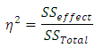where is the sum of squares. measures the proportion of the variation in that is associated with membership of the different groups defined by . is an uncorrected effect size estimate that estimates the amount of variance explained based on the sample, and not based on the entire population. has been suggested to correct for this bias as

See; for example, [13], [14], [15], [16] and [17].

These two measures could be extended to ANOMD as

and

Where measures the proportion of mean differences in that is associated with membership of the different groups defined by. For the above data, Table 11 gives the computations of these measures.

Table 11. The effect sizes for ANOMD and ANOVA tests

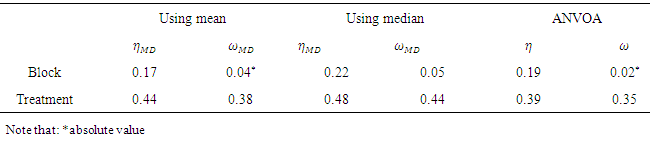
From Table 11, it is interesting to note that the percentage of explained variation using ANOMD for treatment is 44% and 38% while the percentage of explained variation using ANOVA for treatment is 39% and 35%, respectively.

7. Conclusions

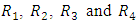
The ANOMD for a randomized complete block was derived by partition the total sum of differences into exact between sum of differences and exact within sum of differences. It had been shown that the TSD had been expressed as a linear combination of the data instead of square.

The ANOMD had important information about the shifts in means and medians that studied by finding the ratios and tested for equal means or medians. Also, it offered a very effective way to find out the shifts in means and medians graphically. Actually, the graph is a very strong point if one can obtain the right conclusion from it. Two effect size measures are extended to ANOMD. These measures are showed that the percentage of explained variation based on ANOMD is more than the percentage of explained variation based on ANOVA.

Also, it is shown that the TSD had not depended on any fixed location and this may make basis for comparisons between more than location measures.