A. C. Akpanta 1, I. E. Okorie 1, N. N. Okoye 2
1Department of Statistics, Abia State University, Uturu, Nigeria
2Agromet Unit, National Root Crops Research Institute Umudike, Nigeria
Correspondence to: A. C. Akpanta , Department of Statistics, Abia State University, Uturu, Nigeria.
| Email: |  |
Copyright © 2015 Scientific & Academic Publishing. All Rights Reserved.
Abstract
This work considered the frequency of monthly rainfall from 1996 to 2011 obtained from National Root Crops Research Institute Umudike in Nigeria. The analysis was based on probability time series modelling approach. The Plot of the original data shows that the time series is stationary and the Augmented Dickey-Fuller test did not suggest otherwise. The graph further displays evidence of seasonality and it was removed by seasonal differencing. The plots of the ACF and PACF show spikes at seasonal lags respectively, suggesting SARIMA (0,0,0) (1,1,1)12. Though the diagnostic check on the model favoured the fitted model, the Auto Regressive parameter was found to be statistically insignificant and this led to a reduced SARIMA (0, 0, 0) (0, 1, 1)12 model that best fit the data and was used to make forecast. Comparison of the actual/observed frequency from July to December 2011 was done with their corresponding forecast values and a t-test of significance showed no significant difference.
Keywords:
Rainfall, Frequency, Time Series, Stationarity, SARIMA
Cite this paper: A. C. Akpanta , I. E. Okorie , N. N. Okoye , SARIMA Modelling of the Frequency of Monthly Rainfall in Umuahia, Abia State of Nigeria, American Journal of Mathematics and Statistics, Vol. 5 No. 2, 2015, pp. 82-87. doi: 10.5923/j.ajms.20150502.05.
1. Introduction
Hitherto, a lot of attention has been directed towards modelling and forecasting the amount of rainfall in various parts of Nigeria. For example: Okorie and Akpanta 2015 [1] modelled extreme monthly rainfall in Ikeja, Nigeria using the Generalized Pareto distribution; Etuk, et al., 2013 [2] identified and established the adequacy of a Seasonal ARIMA (5,1,0)(0,1,1)12 for modelling and forecasting the amount of monthly rainfall in Portharcourt, Nigeria; Edwin and Martins 2014 [3] examined the stochastic characteristics of the Ilorin monthly rainfall in Nigeria using four different modelling techniques (Decomposition, Square root transformation-deseasonalisation, Composite and Periodic Autoregressive) where they compared the results from the various methods employed. In short, so many other works bothering on this subject is almost surely in literature. Unfortunately, knowledge of the amount of monthly or yearly rainfall does not in any way provide information on the frequency of monthly or yearly rainfall respectively, which is also of interest. For example in Agriculture, Research Institutes, Meteorology, Aviation to mention but a few, and has by a long way attracted little or no research attention. However, this paper concisely provides the much needed information on the expected number of times it would rain monthly in Umuahia, the capital of Abia State, using the Box-Jenkins time series modelling technique.
2. Methods
Since the observations of the frequency of monthly rainfall were made sequentially in time and rainfall is an obvious seasonal phenomenon; thus, lending full credence to time series analysis as an appropriate modeling technique to implement. However, emphasis would only be placed on the Seasonal ARIMA (SARIMA) models proposed in Box and Jenkins 1976 [4].
2.1. Seasonal ARIMA (SARIMA) Analysis
A time series is said to be seasonal if there is a sinusoidal or periodic pattern in the series and when this happens the SARIMA model inevitably becomes the choice model. A SARIMA model is only plausible for stationary time series, where stationarity implies constant mean, variance, and autocorrelation functions over time. Unfortunately, many time series data are non-stationary in practice and could be made stationary by a simple differencing exercise. Usually, the first difference is enough to render a non-stationary time series into a stationary one, and the second difference is rarely needed. Most time series plots that fan out suggest the need for variance-stabilizing transformation, e.g. the Box-Cox transformation [5] and the Bartlett’s transformation [6] of the series before considering any data differencing.
2.2. Definition
An ARIMA model is an algebraic statement that describes how a time series is statistically related to its own past.Let 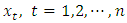 denote a non-stationary seasonal time series which could adequately be modelled by a SARIMA (p, d, q)(P, D, Q)s model defined in operator form
  | (1) |
where  denote the order of the non seasonal and seasonal AR part of the model respectively,
  denote the order of the non seasonal and seasonal MA part of the model respectively,
  denote the number of times the non-stationary and seasonal time series need to be differenced to stationarize and deseasonalize it, respectively. And s in the seasonal model denotes the number of seasons. Interestingly, when
  (1) boils down to SARMA (p, q)(P, Q)S , respectively where both are stationary process, defined by
  | (2) |
respectively, where  are as defined above.
2.3. Steps to SARIMA Modelling
The SARIMA modelling approach is concerned with finding a parsimonious seasonal ARIMA model that describes the underlying generating process of the observed time series. Box and Jenkins [4] established a three step modelling procedure: identification, estimation, and diagnostic checking steps. The identification step is to tentatively choose one or more ARIMA/SARIMA model(s) using the estimated ACF and PACF plots. The ACF plot of the AR (Auto Regressive)/ SAR (Seasonal Auto Regressive) process shows an exponential decay while its PACF plot truncates at lag p /seasonal lag p and diminishes to zero afterwards. The ACF plot of the MA process truncates to zero after lag q/ seasonal lag q while its PACF decays exponentially to zero. The two processes: AR (p)/SAR (P) and MA (q)/SMA (Q), could be combined to form the ARMA (p, q)/SARMA (P, Q) process which has ACF and PACF that decays exponentially to zero. The maximum likelihood estimation method could be used in to estimate the parameters of the identified model(s) in the identification stage. The last diagnostic checking stage involves assessing the adequacy of the identified and fitted models through possible statistically significant test on the residuals to verify its consistency with the white noise process e.g. the Ljung-Box test [7]. Finally, the best fitting model would be selected among other satisfactory, competing models e.g. the information criteria statistics on the basis of the AIC [8] and BIC [9] rule of thumb (Models with the smallest information criterion is the best) and forecast is made with the model of best fit.
3. Results and Discussions
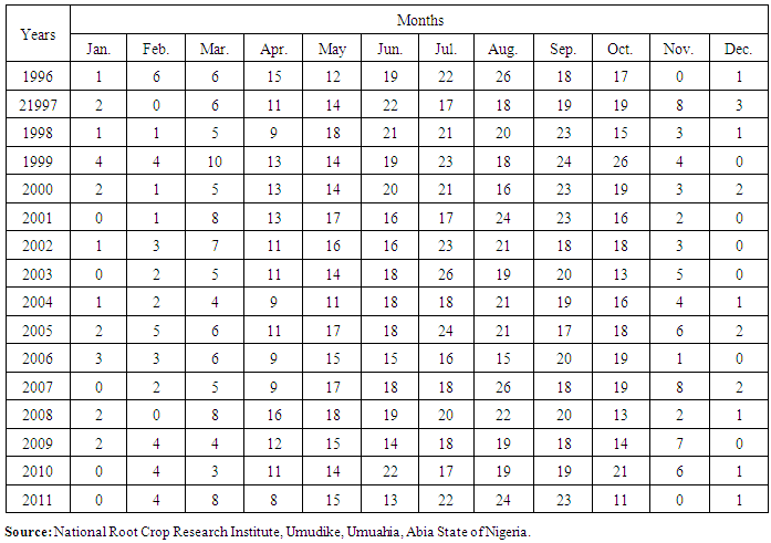
The data (Unpublished in Appendix) on the frequency of monthly rainfall in Umuahia spans from January, 1996 to June, 2011 and was obtained from the National Root Crop Research Institute, Umudike, Umuahia, Abia State of Nigeria. R Statistical Software [10] has been used to perform analysis where results and discussions are presented below. | Figure 1. Time Series Plot (Top Panel), ACF Plot (Centre Panel) and PACF Plot (Bottom Panel) |
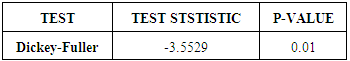
From the plots in Figure 1 it could be seen that the time series plot displays a wave like pattern an evidence of seasonality and no trend is observed which implies that the time series is stationary. The sinusoidal or periodic pattern in the ACF plot is again suggesting that the series has a strong seasonal effect also, the PACF plot is neither suggesting otherwise. In order to verify the stationarity claim of the visual displays we perform the Augmented Dickey-Fuller test [11] with hypothesis H0: The rainfall data is unit root non stationary and H1: The rainfall data is stationary.Table 1. Augmented Dickey Fuller Test
 |
| |
|
Decision: Small p-value 0.01 less than 0.05 is in favour of the alternative hypothesis. Thus, strong evidence against the null hypothesis at 5% level of significance. In order to eliminate the seasonal effect from the time series we subject the data to a seasonal differencing 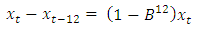 and the data is re-examined visually.All the plots in Figure 2 shows that the first seasonally differenced rain fall series in now well behaved. The pronounced spikes at the first seasonal lags of both the ACF and the PACF plot suggests that a Seasonal ARIMA (SARIMA) (0, 0, 0)(1, 1, 1)12 in operator form
  be fitted to the original rain fall series.Figure 3 shows the overall adequacy of the fitted model. The standardized residual plot shows that the residuals are standard normal distributed on N (0, 1), the ACF plot shows that the residuals are uncorrelated at various lags and the plot of the p-values for the Ljung-Box statistics also supports that the residuals are uncorrelated because the p-values are very large [P-value>0.05(blue dotted line)]. Although the diagnostic plots are in full support of the SARIMA (0, 0, 0)(1, 1, 1)12 model i.e.
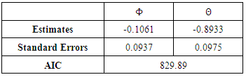
  for the frequency of rainfall data yet, there is a doubt on the goodness of fit of the model because the seasonal AR parameter (Φ) presented in Table 2 has absolute t-value that is less than approximately 2. Thus, dropping this parameter yields SARIMA (0, 0, 0)(0, 1, 1)12 model
 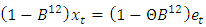 in operator form.
Table 2. Fitted SARIMA (0, 0, 0)(1, 1, 1)12 Model
 |
| |
|
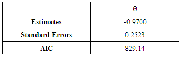
Table 3. Fitted SARIMA (0, 0, 0)(0, 1, 1)12 Model
 |
| |
|
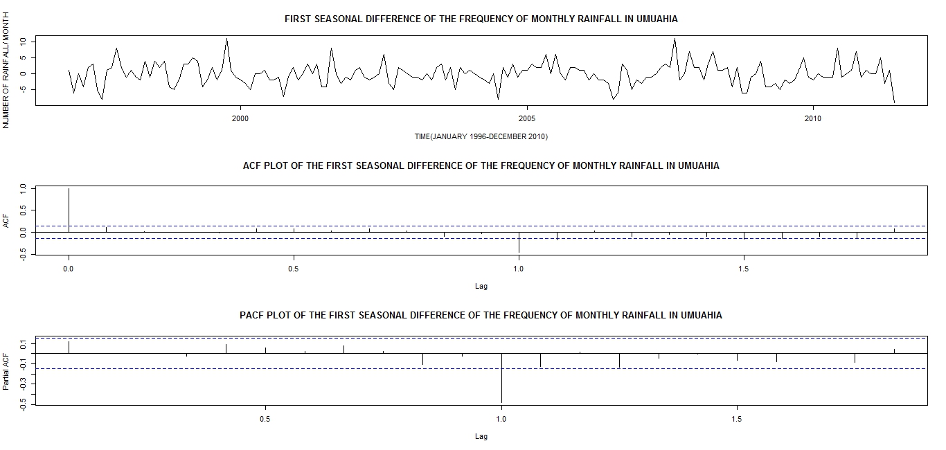 | Figure 2. Plots of Differenced Time Series (Top Panel), its ACF (Centre Panel) and PACF (Bottom Panel) |
There is no noticeable difference between Figure 3 and Figure 4 thus, interpretations remains the same. The seasonal MA parameter (Θ) remains statistically significant because its absolute t-value is larger than 2. The smaller AIC statistic (829.14) of 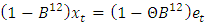 model in comparison to the AIC of (829.89) for
  model implies that the fitted SARIMA (0, 0, 0) (0, 1, 1)12 model provides the best fit to the frequency of monthly rainfall data.
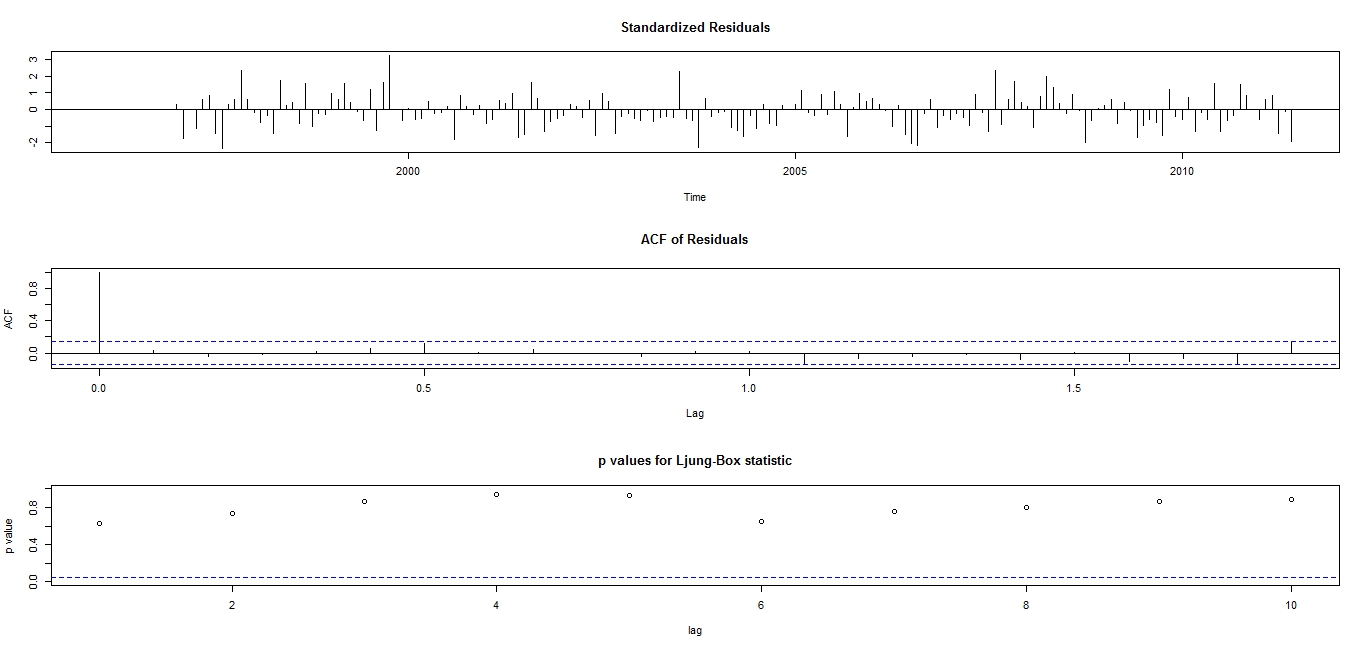 | Figure 3. Diagnostic Plots for the Fitted SARIMA (0, 0, 0)(1, 1, 1)12 |
 | Figure 4. Diagnostic Plots for the Fitted SARIMA (0, 0, 0)(0, 1, 1)12 |
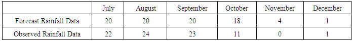
Table 4. SARIMA (0, 0, 0)(0, 1, 1)12 Forecast of the Frequency of Monthly Rainfall in Umuahia Approximated to the Nearest Whole Number
 |
| |
|
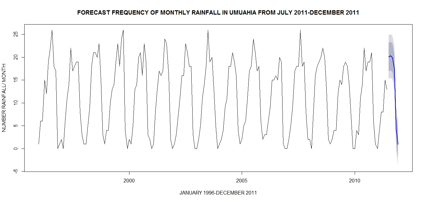 | Figure 5. Plot of the Forecast |
To investigate how satisfactorily the fitted SARIMA (0, 0, 0)(0, 1, 1)12 model has performed in forecasting the future frequency of monthly rainfall in Umuahia we subject the observed and forecast values to a two sample Student's t-test as shown below.Hypothesis: 
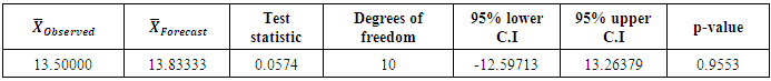
Table 5. Two sample t-test
 |
| |
|
Based on the information in Table 5 we could reasonably conclude at 5% level of significance that there is no statistically significant difference between the observed and forecast frequency of monthly rainfall values. This is because the p-value (0.9553) is greater than 0.05. Alternatively, it could equally be inferred from the 95% confidence interval (-12.59713, 13.26379) because the interval contains zero. Thus, the SARIMA (0, 0, 0) (0, 1, 1)12 model has done a good job in forecasting the Frequency of monthly rainfall in Umuahia and is therefore recommended for this task.
4. Conclusions
In this study, the frequency, not the amount, of monthly rainfall from 1996 to 2011 obtained from the National Root Crop Research Institute (NRCRI) Umudike in Nigeria, is analysed using probability time series modelling approach. The Plot of the original data in Figure 1 shows that the time series is stationary and has evidence of seasonality. The Augmented Dickey-Fuller test in Table 1 confirmed the stationarity claim. Seasonal differencing was done to remove the seasonal effect. SARIMA modelling of the data was upheld after duely following the conventional three steps of identification, estimation and diagnostic checking procedures established by Box and Jenkins. This resulted in obtaining SARIMA (0, 0, 0) (1, 1, 1)12. However, the seasonal Auto Regressive parameter in Table 2 was found to be statistically insignificant and this consequently led to a new model SARIMA (0, 0, 0) (0, 1, 1)12 that best fit the data and was used to make forecast. Comparison of the actual/observed frequency from July to December 2011 was done with their corresponding forecast values and a t-test of significance showed no significant difference.
Appendix
Table 6. Frequency of Monthly Rainfall in Umuahia from 1996 to 2011
 |
| |
|
References
| [1] | Okorie I. E and Akpanta A. C Threshold Excess Analysis of Ikeja Monthly Rainfall in Nigeria: International Journal of Statistics and Applications, February 2015. - 1 : Vol. 5. Pp. 15-20. |
| [2] | Etuk H. E, Moffat U. I and Chims E. B. Modelling Monthly Rainfall Data of Portharcourt, Nigeria by Seasonal Box-Jenkins Method: International Journal of Sciences, 2013. - 7: Vol. 2. |
| [3] | Edwin A. and Martins O. Stochastic Characteristics and Modelling of Monthly Rainfall Time Series of Ilorin, Nigeria: Open Journal of Modern Hydrology, 2014. - Vol. 4. - pp. 67-69. - doi: 10.4236/ojmh.2014.43006. |
| [4] | Box G.E.P. and Jenkins G.M. Time series Analysis, Forecasting and Control . San Francisco: Holden-Day, 1976. |
| [5] | Box G. E. P. and Cox D. R. An analysis of transformations . JRSS. - 1964. - Vol. B 26. - pp. 211–246. |
| [6] | Bartlett M.S. The Use of Transformations, Biometrika, 3: (1947), 39-52. |
| [7] | Ljung G. M. and Box G. E. P. On a Measure of Lack of Fit in Time Series Models. Biometrika. - 1978. - Vol. vol. 65. - pp. 297. |
| [8] | Akaike H. A New Look at the Statistical Model Identification. Annals of Statistics: IEEE Trans. Automat. Contr., 1974. - Vols. Ac-19. - pp. 716-723. |
| [9] | Schwarz G. Estimating the Dimension of a Model. Annals of Statistics. - 1978. - Vol. 6. - pp. 461-464. |
| [10] | R Development Core Team R: A language and environment for statistical computing // R Foundation for Statistical Computing. - Vienna, Austria: [s.n.], 2014. - 3-900051-07-0. |
| [11] | Dickey D. A. and Fuller W.A. Autoregressive Time Series with a Unit Root. Journal of American Statistical Association. - 1979. - Vol. 74. - pp. 427-431. |
 Abstract
 Reference
 Full-Text PDF
 Full-text HTML