Stephen Ehidiamhen Uwamusi
Department of Mathematical Sciences, Kogi State University, Anyigba, Nigeria
Correspondence to: Stephen Ehidiamhen Uwamusi , Department of Mathematical Sciences, Kogi State University, Anyigba, Nigeria.
| Email: |  |
Copyright © 2015 Scientific & Academic Publishing. All Rights Reserved.
Abstract
The paper discusses the graph completion inclusion isotone for interval least squares problem wherein, incorporated the Tikhonov regularization for resolving the recurrent problem of ill-conditioning for the resulting interval linear least squares using quadratic polynomial fit. It is established that convergence of interval operators to the described interval least squares problems implies convergence in the tempered distribution of interval data in the sense of [2]. The open Question of Completeness of graph in Banach Space Topology is addressed and estimate of eigenvalues to the interval matrix was given further interpretation using ideas of [24] which has great importance in the study of growth rate of a system. Numerical example is demonstrated with described methods.
Keywords:
Least squares problem, Graph inclusion isotone, Banach space, Tempered distribution, Circular interval arithmetic, Interval matrix eigenvalues
Cite this paper: Stephen Ehidiamhen Uwamusi , Graph Completion Inclusion Isotone for Interval Least Squares Equation, American Journal of Mathematics and Statistics, Vol. 5 No. 1, 2015, pp. 24-31. doi: 10.5923/j.ajms.20150501.04.
1. Introduction
The paper considers graph completion inclusion isotone for least squares problem with uncertain data. The closed graph theorem in the sense of [1], and [2] for instance gives a basic result that characterizes continuous functions in terms of their graphs. For any function  we define the graph
  , as the map
  to be the Cartessian product
 .There is a metric topology for which is defined
 . When
  is Cauchy, for
  it follows that
  in
in  as
as . In other words, for a closed graph F, it holds that
  forcing
 implying the graph of
  is enclosed by the convex hull of control points. In a nutshell, a graph
  is continuous at the point
  if it pulls open sets back to open sets and carries open sets over to open sets.Fundamental to this discussion are the basic principles of advanced topology. Good reference texts may be [1], [3] and [4]. Following [1], a linear map F from a linear topological space X to a linear topological space Y will be called bounded if it maps bounded sets to bounded sets. A map which is a linear topological space X to a linear topological space Y will be called sequentially continuous if for every sequence
  converging to some point x of E has a bounded envelope and such a sequentially continuous map is ultrabarrelled [1]. A function F is called approxable in the sense of [5] if for a multi valued mapping
  for every
  there is continuous single valued mapping
  with graph
  . A function
  is said to be upper semi-continuous at
  if for any neighbourhood
  of
of  there exists a neighbourhood
  of
of  such that
  . A similar definition goes for a lower semi continuous function.By reasons due to recurrence and category theorem, the map
  has a measure preserving homeomorphism and hence its set of recurrent point is residual and of full measure. In other words it can be said that such a map has a generic measure preserving homeomorphism whose square has a dense orbit. In some cases one often comes across some functions with distortions at some points which necessitate the following definition.Definition 1.1, [6]. Let
  be a map between two locally Euclidean metric spaces. The quantity
  , is called the radius
  distortion of
  at x.As a consequence following, we introduce the nonlinear system of equation
 | (1.1) |
where  , m>n,
  is an interval vector. It is supposed that the function F has at least
  where
where  . Therefore, in a Frechet space E, every continuous linear map from a Frechet space E into F has a closed range and such a map is finite dimensional. Applications of nonlinear systems for example are well documented in the work of [7] which includes the following: Aircraft stability problems, Inverse Elastic rod problems, Equations of radiative transfer, Elliptic boundary value problems, Power flow problems, Distribution of water on a pipeline, Discretization of evolution problems using implicit schemes, Chemical plant equilibrium problems and, Nonlinear programming problems. We often adopt the concept of divided difference from a univariate function which is extended over to multivariate vector valued function by defining slope as
  , provided that F is differentiable on the line
  .Motivated by the above details, we state the following:Lemma 1.1, [8]. Let
  be convex and let
  be continuously differentiable in D.(i) If
  then
then  (This is a strong form of Mean-value theorem);(ii) if
  then
then  and
and  (This is a weak form of Mean-value theorem);(iii) if
  is Lipschitz continuous in D, that is the relation
  holds for some
  , then
  (This is truncated Taylor expansion with remainder term).It is a result to follow up to the discussion that we have the following theorems.Theorem 1.1, [9]. Suppose
  has an F-derivative at each point of an open neighbourhood of
 . Then,
  is strong at x if and only if
  is continuous at
  .Because system 1.1 is over determined, we often transform to a linear system by the process of 2-norm assuming that the Jacobian matrix
  which is rectangular exists in the form
 | (1.2) |
This operator is required to be everywhere defined that also holds verbatim in Banach space, provided its graph  is closed in
  with respect to its product topology.Of paramount interest to us is a mapping that is balanced and absorbent whose inductive limit is ultra barrelled for which contraction mapping of Newton-Mysovskii theorem follows: Theorem 1.2, [9]. Supposing that
  is F-differentiable on a convex set
  and that for each
  is non-singular and satisfies
  . Assuming further that
  such that
  ;
;  and
and  for which
 . Then the iterated contraction of Newton operator is in the form:
 | (1.3) |
which remains in  and converges to a solution
  of
of  .Moreover,
 where
where  .We expect the weak pre-image
  and the strong pre-image
  coincide simultaneously such that the orbit of F is a sequence
  for which
  | (1.4) |
holds good that  be coercive and a local homeomorphism of
  to itself, every zero of
  is in the intersection of convex hull with the hyper plane
 .As a result of equation 1.4 the norm reducing property of Newton operator for system 1.1 is given by
  for k=0,1,.., .The quantity
  will be called the order of convergence for
  assuming the limit exists which is again equal to the R-Order of convergence of [9].The rest part in the paper is arranged as follows: Section 2 discusses what is meant by the statistical meaning of the matrix
  . Section 3 describes completeness of graph in Banach space topology. Procedure for estimating eigenvalues of interval Jacobian matrix formed the basis of discussion in chapter 4. Section 5 in the paper gives numerical illustration of what has been discussed in previous sections.
2. The Statistical Meaning of the Matrix  and Its Applications
Henceforth, we adopt that the matrix A denotes the matrix A(x). In line with ideas expressed in [10] we give the statistical meaning to the matrix . We note that the components
  are independent, normally distributed random variable with mean
  and all having the same variance
  which we describe in the form:
 ,
,  Therefore setting
  there holds that
  The covariance matrix of the random vector y is given by
 . The first moments are
  and
and . For a rectangular matrix A for which
  is non singular Nuemaier [11] using
  decomposition proved that
  for all x.Following [12], it was proved that over any field,
 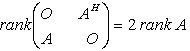 and that
 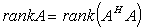 holds over any field of characteristic 0. This means computing least squares solution or bounding the errors of computations are not defined over an arbitrary field. It thus holds that
  and that
 .We shall be interested in the least squares problem where the coefficient matrix and right hand vector assume some kind of noise often known as white noise. This situation leads to what is called Total Least Squares Problem (TLS) whereby, tempered distribution to the coefficient matrix A is
 , and to the vector y by
  respectively for which holds
 | (2.1) |
Subject to  | (2.2) |
The expression  is the usual Frobenius norm which coincides with
  in the classical Banach space. In its simplest form, the linear inverse problem [13], [14] to which the least squares problem belongs was described in the form:
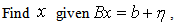 | (2.3) |
where,  represents
 ,
,  , and
, and  is the realization of random noise. Thus when B is invertible the linear system 2.3 is said to be well posed whereas it is ill-posed when B is not invertible.As a result the minimum
  -norm of the residual is given by
 | (2.4) |
Where, it is understood that  is the norm on
  with unit ball defined by
  ..By substituting (2.4) into (1.1) we have that
 | (2.5) |
In equation 2.5, the second term  dominates in the ill-posed problem when the uncertainty is high thereby making
  practically useless in most cases of applications. This means that the induced map
  is open, nearly continuous, and nearly open if and only if
  has the same ill-posed property, [1]. Therefore via interval arithmetic this problem has been addressed [15].We expect that both
  and
and  be closed in the
  topology [1] so that,
  convergence implies convergence in the tempered distribution for which any neighbourhood
  in the metric space
  holds for
  satisfying system 1.1.As pointed by some schools of thought, one drawback of Tikhonov regularization is that it tends to produce a solution that is often excessively smooth in image processing for which this method results in loss of sharpness. Nevertheless, the classical Tikhonov regularization method for minimizing
  has the solution as
 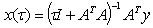 in the sense of [16]. The equation that determines
  in the restructured least squares sense was given by
  | (2.6) |
where  is well defined.Thus when
  the optimal solution is given by
 Where
Where  are the unique optimal point to the problem minimize
 Note that
  and
and  .Since
  and
and  is rank one, it holds that
  . This forces
 .Equation 2.6 is used when there is no perturbation in y. In case of total least squares the solution to the perturbed least squares equation 2.1 is given by the
  | (2.7) |
where  is the smallest singular value of
  , ([ 17], e.g.,). In most applications of interest we often perturb the matrix B such that perturbation
  satisfies the condition that
  and
and  | (2.8) |
Because of equation 2.8, it follows that | (2.9) |
Where we used the fact that , and
, and . The matrix
  is the Pseudo-Penrose inverse of
  .As a result of equations 2.8 and 2.9 and in view of equation 2.7, it can be deduced that
  | (2.10) |
The actual value of  as well as
  is obtained in the form
 | (2.11) |
 | (2.12) |
Therefore when the matrix B is perturbed by  , from well known result [18] there holds the estimate
 | (2.13) |
3. The Question of Completeness of graph in Banach Space Topology
We are interested in the regularity property of graph that is equated to openness which relates regularity to inversion problems. By this we mean regularity of set valued maps, [19] for which openness and inversion properties of equation 1.1 form the basis of investigation. Inverse mapping theorem asserts that the inverse of an invertible bounded linear operator between Banach spaces is a continuous map.As is well known, a complete metric space cannot be written as a countable union of nowhere dense sets. The Baire Category theorem provides that , an indication that F is open around
 and
and  is the open
  -neighbourhood of x in
  . That is,
 | (3.1) |
Fundamentally, what is required is the graph completion operator that is inclusion isotone with respect to functional argument. That is, the Hausdorff continuous operator  satisfying the inclusion
  which is Dedekind order complete
  with respect to point wise defined partial ordering. As it were, we also assume that
  finite algebra of measurable sets holds verbatim. As is standard, the completeness of the graph suffices to show
 . That
  implies that it is absolutely summable, which is that,
  . It follows that
  , a consequence of Banach space. We note in passing that if
  is not Hausdorff, an extreme point is not a supporting set.
4. Distribution of Eigenvalues of the Jacobian Matrix
A very important issue in engineering application has always been the occurrence of a saddle node bifurcation , Hopf bifurcation or solution near such bifurcation points,[20]. Denoting A(x) as the Jacobian matrix of partial derivative of F(x) assuming that system 1.1 is of order n, the eigenvalues of A(x) is represented by . Let
. Let  which does not contain eigenvalues of A other than
 . Then
  . The number of zeros
  inside
  is given by argument principle [10]
 | (4.1) |
Thus  , the integral is analytic function of
  and of
  .In other words assuming
  is analytic in the sense of [21] inside and on a closed contour
  which encloses
  , then
  will be defined by the equation
 | (4.2) |
Supposing the eigenvalues are able to discriminate their goals such that | (4.3) |
And assuming further one can find  , then
  is called a saddle-node bifurcation point of the nonlinear system of equation 1.1. Furthermore, if A(x) has a pair of conjugate eigenvalues passing the imaginary axis while the other eigenvalues have negative real parts, then is called a Hopf bifurcation point.The solution to nonlinear system 1.1 is said to be stable if the eigenvalues of A(x) have negative real part.Using [17], the 2-norm,
  for unsymmetrical matrix
  is the numerical abscissa
  where in its application, the behaviour of
  may be different in the initial, transient, and asymptotic phase. In other words, the asymptotic behaviour depends on
  as
as  whenever
 . In any case, the bound given by
  is the best possible.The cosine angle between two matrices
  using Frobenius inner product is given by
  | (4.4) |
Where  , [20] and
  is often used in practice in which case
 | (4.5) |
The relative condition numbers for the matrix sine and cosine in the sense of [22] satisfy  | (4.6) |

 After all these, the estimation of eigenvalues of interval Jacobian matrices will be computed. Popular such methods for estimating bounds of eigenvalues have been the Gesrchgorin disks or Ovals of Cassini, [23]. Unfortunately the bounds these methods produce for the case of interval matrices had been known to be too wide for any meaningful uses. We proceed in the same spirit similar to [24] as well as [25] to provide realistic bounds for eigenvalues of interval matrices coming from the Jacobian of system 1.1.For general treatment of eigenvalues, consider unsymmetric matrices of order n where for clarity, we adopt the following notation:
 ,
,  , and after verification of
  Rohn showed that a necessary and sufficient condition for
  to be eigenvalue of interval matrix [A] is that
  is singular. That is to say a number
  is an eigenvalue of
  if the two conditions below can be verified
 then
then  is a real eigenvalue of A
 then
then  is not a real eigenvalue of A[22] proved that eigenvalues of symmetric interval matrix A lie in the interval
  where
where 
 .The
.The 
 respectively denote minimal and maximal eigenvalue of
  . Let us take note that a rectangular matrix
  has full column rank if it possible to compute
  . For example the upper end point
  of the desired interval indicates how fast a population can grow or how fast a disease can spread in any experimental data analysis. As pointed out by [24] the estimated eigenvalue bound provided by Rohn’s method has the drawback of still not being empty even when the set of eigenvalues is empty.
5. Numerical Examples
Problem 1.Consider a set of two-dimensional points :
: Using quadratic polynomial fit for the data set and if we take notice of the resulting Vandermode matrix, and using MATLAB version 2007, the solution for equation 2.1 is obtained as
 , with eigenvalues to the symmetric matrix
  .Providing solution to the interval linear system a procedure earlier described in [15] applies. As a consequence, we omit repeating it here.We are concerned with providing estimates of the eigenvalues computed for interval matrix which was derived from the above statistical data set
 And this was computed to be
 .Using Rohn’s method [24] we also obtained eigenvalues bound to be
 Using a 20% impurity as data noise we obtained bounds for eigenvalues of interval matrix as
  With condition number
  and it can be seen that matrix eigenvalues may be affected by level of impurities in the statistical data set.
6. Conclusions
The paper studied graph completion operator for interval least squares problem. We discussed the statistical meaning of the matrix  obtained from the statistical data entries of observation. It is shown that convergence of inverse operators for the resulting regularized Tikhonov parameter implies convergence in the tempered distribution of data noise wherein the earlier procedure described in [15] is applicable. Our emphasis was placed on estimating interval matrix which has great applications in the study of growth rate of a system which was applied on statistical least squares problem. As pointed out by [24] the estimated eigenvalue bound provided by Rohn’s method [24] has the drawback of still not being empty even when the set of eigenvalues may be empty as demonstrated by numerical example. This may be found useful in both Scientific and Engineering designs.
References
| [1] | Iyahen S.O (1998). The Closed Graph Theorem, Osaruwa Educational Publications, First Edition, Benin City. |
| [2] | Wikipedia (2014). Closed graph theorem. The free encyclopaedia, Mozila Fireworks. |
| [3] | Mane R (1987). Ergodic Theory and Differentiable Dynamicss, Springer-Verlag. |
| [4] | Oxtoby JC (1980). Measure and Category, Springer-Verlag. |
| [5] | Schodl P and Neumaier A (2010). Continuity notions for multivalued mappings with possibly disconnected images. Reliable Computing, pp 1-18. |
| [6] | Kelner JA (2006). Spectral partitioning, eigenvalue bounds, and circle packings for graphs of bounded genus, SIAM J. Comput Vol. 35 No 35, PP. 882-902. |
| [7] | Martinez JM (1994). Algorithms for solving nonlinear systems of equations, Continuous optimization: the state or art (In edt. Spedicato E), Kluwer, 81-108. |
| [8] | Neumaier A (2000). Introduction to Numerical analysis, Cambridge University Press, Cambridge. |
| [9] | Ortega JM and Rheinboldt WC (2000). Iterative solution of nonlinear equations in several variables, SIAM, Philadelphia. |
| [10] | Stoer J and Bulirsch R (1983). Introduction to Numerical Analysis, Springer-Verlag, New York. |
| [11] | Neumaier A (2004). Complete search in continuous global optimization and constraint satisfaction. A Chapter for Acta Numerical 2004 (A. Iserles, ed.), Cambridge University Press. |
| [12] | Bini D and Pan V (1994). Polynomial and matrix Computations Vol. 1: Fundamental algorithms, Birkhauser, Boston. |
| [13] | Stefan W. (2008). Total Variation regularization for linear Ill-posed inverse problems: Extensions and application, PhD thesis, Graduate College, Arizona State University , USA. |
| [14] | Ferson S, Kreinovich V, Hajagos J, Oberkamp W and Ginzburg L (2007). Experimental uncertainty estimation and statistics for Data having interval uncertainty. SAND 2007-0939 Unlimited release. Available online at http//:www.amas.com/inststats.pdf |
| [15] | Uwamusi SE (2014). Regularization of Non-smooth function whose Jacobian is nearly singular or singular, America International Journal of Contemporary Scientific Research-180, ISSN 2349-4425. Available in www.americanij.com |
| [16] | El-Ghaoui L and Lebret H (1977). Robust solutions to least-squares problems with uncertain data, SIAM J. Matrix Anal. Appl Vol 18(4) pp 1035-1064. |
| [17] | Bjorck A, (2009). Numerical methods in Scientific Computing Vol. 2, SIAM, Philadephia. |
| [18] | Hargreaves G (2006). Computing the condition number of Tridiagonal and diagonal-plus semiseprable matrices in linear time, SIAM J. Matrix Anal. Appl, 27(30, PP. 801-820. |
| [19] | Borwein JM and Zhuang DM (1988) Variable necessary and sufficient conditions for openness and regularity of set-valued and Single-valued maps, Journal of Mathematical analysis and applications 134, 441-459. |
| [20] | Kelly CT, Qi L , Tong X and Yin H (2011). Finding a stable solution of a system of Nonlinear equations arising from Dynamic systems, Journal of Industrial and Management Optimization, 7(2), 297. |
| [21] | Tarazaga P (1989). More estimates for eigenvalues and singular values, TR 89-6. |
| [22] | Higham NJ (2009). Functions of Matrices: Theory and Computation, SIAM Philadelphia. |
| [23] | Varga RS (2000). Matrix iterative analysis, Springer Computational Mathematics, Second Edition, New York. |
| [24] | Rohn J (2005). A Handbook of results on interval analysis, Czech Academy of Sciences, Prague, Czech Republic, European Union. |
| [25] | Hadlik M, Daney D and Tsigaridas EP (2008). Bounds on eigenvaues and singular values of interval matrices, INRIA Institut National Recherche en infomatique et en automatique . |
 Abstract
 Reference
 Full-Text PDF
 Full-text HTML