Etebong P. Clement
Department of Mathematics and Statistics University of Uyo, Akwa Ibom State, Nigeria
Correspondence to: Etebong P. Clement, Department of Mathematics and Statistics University of Uyo, Akwa Ibom State, Nigeria.
| Email: |  |
Copyright © 2014 Scientific & Academic Publishing. All Rights Reserved.
Abstract
A Statistical Time Series model is fitted to the Chemical Viscosity Reading data. Comparison with the original models fitted to the same data set by Box and Jenkins is made using the Normalized Bayesian Information Criterion (BIC) and analysis and evaluation are presented. The analysis proved that the proposed model is superior to the Box and Jenkins models.
Keywords:
ARIMA, Bayesian Information Criterion (BIC), Box-Jenkins Approach, Ljung-Box Statistic, Time Series Analysis
Cite this paper: Etebong P. Clement, Using Normalized Bayesian Information Criterion (Bic) to Improve Box - Jenkins Model Building, American Journal of Mathematics and Statistics, Vol. 4 No. 5, 2014, pp. 214-221. doi: 10.5923/j.ajms.20140405.02.
1. Introduction
The Box-Jenkins approach to modeling ARIMA (p,d,q) processes is adopted in this work. The original Box-Jenkins modeling procedure involved an iterative three-stage process of model selection, parameter estimation and model diagnostic checking. Recent explanations of the process (e.g. [1]) often include a preliminary stage of data preparation and a final stage of model application (or forecasting). Although originally designed for modeling time series with ARIMA (p,d,q) processes, the underlying strategy of Box-Jenkins is applicable to a wide variety of statistical modeling situations. It provides a convenient framework which allows an analyst to find an appropriate statistical model which could be used to answer relevant questions about the data.ARIMA models describe the current behaviour of variables in terms of linear relationships with their past values. These models are also called Box-Jenkins Models on the basis of these authors’ pioneering work regarding time series forecasting techniques. An ARIMA model can be decomposed into two parts [2]. First, it has an integrated (I) component (d) which represents the order of differencing to be performed on the series to attain stationarity. The second component of an ARIMA consists of an ARMA model for the series rendered stationary through differentiation. The ARMA component is further decomposed into AR and MA components [3]. The Auto Regressive (AR) components capture the correlation between the current values of the time series and some of its past values. For example, AR (1) means that the current observation is correlated with its immediate past values at time . The moving Average (MA) component represents the duration of the influence of a random (unexplained) shocks. For example, MA (1) means that a shock on the value of the series at time t is correlated with the shock at time
 . The autocorrelation functions (acf) and partial Autocorrelation functions (pacf) are used to estimate the values of p and q.
2. Methodology
The Box - Jenkins methodology adopted for this work is widely regarded as the most efficient forecasting technique, and is used extensively. It involves the following steps: Model identification, model estimation, model diagnostic check and forecasting [4].
2.1. Model Identification
The foremost step in the process of modeling is to check for the stationarity of the time series data. This is done by observing the graph of the data or autocorrelation and the partial autocorrelation functions [1]. Another way of checking for stationarity is to fit the first order AR model to the raw data and test whether the coefficients  is less than one.The task is to identify an appropriate sub-class of model from the general ARIMA family.
 | (1) |
which may be used to represent a given time series. Our approach will be:(i) To difference  as many times as is needed to produce stationarity.
  | (2) |
where | (3) |
(ii) To identify the resulting ARIMA process. Our principal tools for putting (i) and (ii) into effect will be the autocorrelation and the partial autocorrelation functions.Non-stationary stochastic process is indicated by the failure of the estimated autocorrelation functions to die out rapidly. To achieve stationarity, a certain degree of differencing (d) is required. The degree of differencing (d), necessary to achieve stationarity is attained when the autocorrelation functions of  | (4) |
die out fairly quickly.The autocorrelation function of an AR (p) process tails off, while its partial autocorrelation function has a cut off after lag p. Conversely, the acf of a MA (q) process has a cut off after lag q, while its partial autocorrelation function tails off. However, if both the acf and pacf tail off, a mixed ARMA (p,q) process is suggested. The acf of a mixed ARMA (p,q) process is a mixture of exponentials and damped sine waves after the  lags. Conversely, the pacf of a mixed ARMA (p,q) process is dominated by a mixture of exponentials and damped sine waves after the first
  lags.
lags.
2.2. Model Estimation
Preliminary estimates of the parameters are obtained from the values of appropriate autocorrelation of the differenced series. These can be used as starting values in the search for appropriate least square estimates. In practice not all parameter in the models are significant. The ratios  | (5) |
may suggest trying a model in which some of the parameters are set to zero [5]. Then, we need to re-estimate the model after each parameter is set to zero.
2.3. Diagnostic Check
The diagnostic check is a procedure that is used to check residuals. The residual should fulfill the models assumption of being independent and normally distributed. If these assumptions are not fulfilled, then another model is chosen for the series. We will use the Ljung-Box test statistic for testing the independency of the residuals. Also, statistical inferences of the parameters and the goodness of fit of estimated statistical models will be made.
2.3.1. Ljung – Box Statistics
[6] statistic tests whether a group of autocorrelations of a time series are less than zero. The test statistic is given as:  | (6) |
where T: number of observations s: length of coefficients to test autocorrelation  Autocorrelation coefficient (for lag k)The hypothesis of Ljung - Box test are:
 Residual is white noise
  Residual is not white noiseIf the sample value of
  exceeds the critical value of a
  distribution with
  degrees of freedom, then at least one value of
  is statistically different from zero at the specified significance level.
2.3.2. Bayesian Information Criterion (BIC)
In statistics, the Bayesian information criterion (BIC) or Schwarz criterion (also SBC, SBIC) is a criterion for model selection among a finite set of models. It is based, in part, on the likelihood function, and it is closely related to Akaike information criterion (AIC). When fitting models, it is possible to increase the likehood by adding parameters, but doing so may result in over fitting. The BIC resolves this problem by introducing a penalty term for the number of parameters in the model. The penalty term is large in BIC than in AIC.The BIC was developed by Gideon E. Schwarz [7], who gave a Bayesian argument for adopting it. It is closely related to the Akaike information criterion (AIC). In fact, Akaike was so impressed with Schwarz’s Bayesian formalism that he developed his own Bayesian formalism, now often referred to as the ABIC for “a Bayesian Information Criterion” or more casually “Akaike’s Bayesian information criterion” [8].The BIC is an asymptotic result derived under the assumptions that the data distribution is in the exponential family. Let  : The observed data;
 number of data points in
  the numbers of observations, or equivalently the sample size;
 : The numbers of free parameters to be estimated.If the estimated model is a linear regression,
  is the number of regressors, including the intercept;
  The probability of the observed data given the number of parameters; or, the likelihood of the parameters given the dataset;
  maximized value of the likelihood functions for the estimated model.The formula for the BIC is:
 | (7) |
with the assumption that the model errors or disturbances are independent and identically distributed according to normal distribution and that the boundary condition that the derivative of the log likelihood with respect to the true variance is zero, this becomes (up to an additive constant, which depends only on  and not on the model [9].
 | (8) |
where  is the error variance.The error variance in this case is defined as
 | (9) |
One may point out from probability theory that  is a biased estimator for the true variance,
  Let
Let  denote unbiased form of approximating the error variance. It is defined as:
  | (10) |
Additionally, under the assumption of normality the following version may be more tractable  | (11) |
Note that there is a constant added that follows from transition from log-likelihood to  however, in using the BIC to determine the “best” model the constant becomes trivial.Given any two estimated models, the model with the lower value of BIC is the one to be preferred. The BIC is an increasing function of
  and an increasing function of
  . That is, unexplained variations in the dependent variable and the number of explanatory variables increase the value of BIC. Hence, lower BIC implies either fewer explanatory variables, better fit, or both. The BIC generally penalizes free parameters more strongly than does the Akaike Information Criterion, though it depends on the size of
  and relative magnitude of
  and
and  .It is important to keep in mind that the BIC can be used to compare estimated models only when the numerical values of the dependent variable are identical for all estimates being compared. The models being compared need not be nested, unlike the case when models are being compared using an
  or likelihood ratio test.
2.3.2.1. Characteristic of the Bayesian Information Criterion
It is independent of the prior or the prior is “vague” (a constant). It can measure the efficiency of the parameterized model in terms of predicting the data. It penalizes the complexity of the model where complexity refers to the number of parameters in models.It is approximately equal to the minimum description length criterion but with negative sign.It can be used to choose the number of clusters according to the intrinsic complexity present in a particular dataset. It is closely related to other penalized likelihood criteria such as RIC and the Akaike Information Criterion (AIC).
2.3.2.2. Implications of the Bayesian Information Criterion
BIC has been widely used for model identification in time series and linear regression. It can, however, be applied quite widely to any set of maximum likelihood-based models. However, in many applications (for example, selecting a black body or power law spectrum for an astronomical source), BIC simply reduces to maximum likelihood selection because the number of parameters is equal for the models of interest.
3. The Analysis of Data
Having discussed some basic concepts and theoretical foundation of time series that will enable us analyze the data. We now present a step by step analysis of our dataset of Series D.
3.1. Model Identification
The graphical plot of the original series of the chemical process viscosity Reading: (Every Hour) is given in figure 1. It is observed that, the series exhibits non-stationary behaviour indicated by its growth.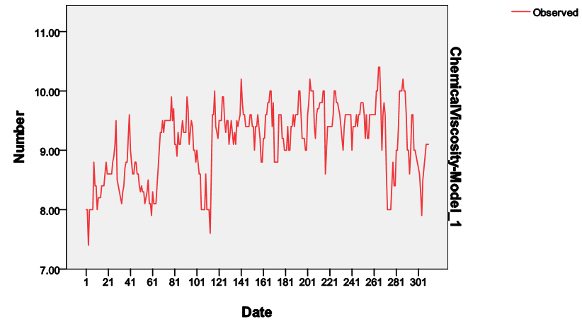 | Figure 1. Graph of original series  |
The sample autocorrelations of the original series in figure 2 failed to die out quickly at high lags, confirming the non-stationarity behaviour of the series, which equally suggests that transformation is required to attain stationarity. Consequently, the difference method of transformation was adopted and the first difference  of the series was made. The plot of the stationary equivalent is given in figure 3 while the plots of the autocorrelation and partial autocorrelation functions of the differenced series are given in figure 4 and figure 5 respectively.
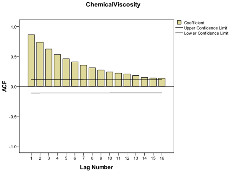 | Figure 2. Plot of Autocorrelation Functions of the Original Series  |
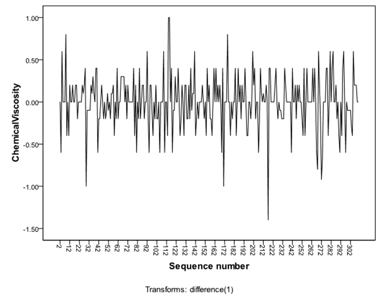 | Figure 3. Graph of the Differenced Series D (-1) |
 | Figure 4. Plot of the Autocorrelation functions of the differenced Series |
 | Figure 5. Plot of the Partial Autocorrelation functions of the differenced Series |
The autocorrelation and partial autocorrelation functions of the differenced series indicated no need for further differencing as they tend to be tailing off rapidly. They also indicated no sign of seasonality since they do not repeat themselves at lags that are multiples of the number of periods per season.Using figure 4 and figure 5, the differenced series will be denoted by  for
for  where
where  It is observed that both the autocorrelation and partial autocorrelation functions of
  are characterized by correlations that alternate in sign and which tend to damp out with increasing lag. Consequently, a mix autoregressive moving average of order (1, 1, 1) was proposed since both the autocorrelation and partial autocorrelation functions of the
  seem to be tailing off.Thus, using equation (1), the proposed model is an ARIMA (1,1,1).
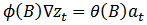 | (12) |
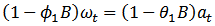 | (13) |
 | (14) |
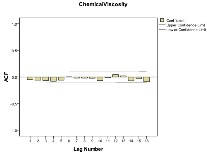
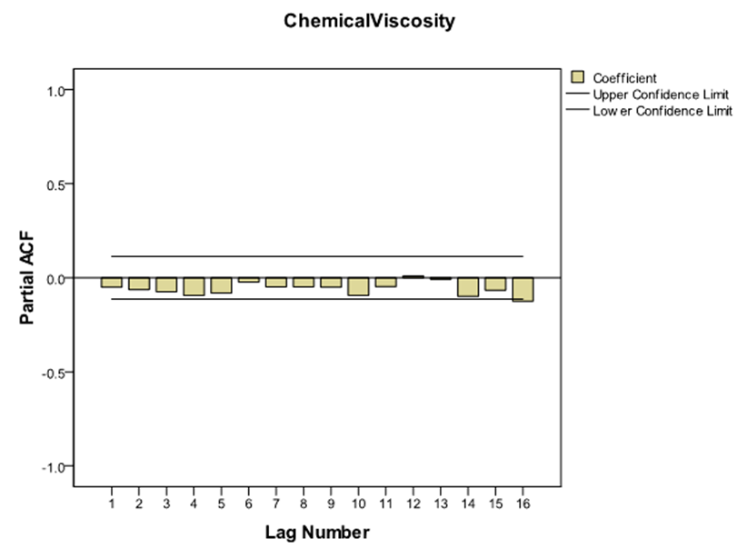
The plot of the autocorrelation and partial autocorrelation functions of the residuals from the tentatively identified ARIMA (1, 1, 1) model are given in figure 6.
3.2. Estimation of Parameters
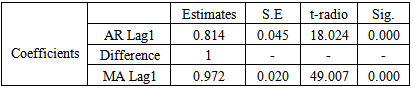
Having tentatively identified what appears to be a suitable model, the next step is to obtain the least squares estimates of the parameters of the model. The SPSS 17 Expert Modeler was used to fit the model to the data. The coefficient of both the AR and the MA were not significantly different from zero with values of 0.814 and 0.972 respectively. This model enables us to write the model equation as: | (15) |
That is, the AR coefficient  was estimated to be 0.814 with standard error of 0.045 and a t-ratio of 18.024 while the MA coefficient θ was estimated to be 0.972, with standard error of 0.020 and a t-ratio of 49.007.For this model Q = 9.746. The 10% and 5% points of chi-square with 16 degree of freedom are 23.50 and 26.30 respectively. Therefore, since Q is not unduly large and the evidence does not contradict the hypothesis of White Noise behaviour in the residuals, the model is very adequate and significantly appropriate.
3.3. Model Diagnostic Check
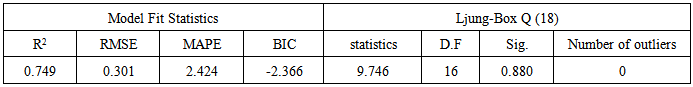
It is concerned with testing the goodness of fit of the model. From plots of the residual acf and pacf, it can be seen that all points are randomly distributed and it can be concluded that there is an irregular pattern which means that the model is adequate. Also, the individual residual autocorrelations are very small and are generally within  significance bounds. Also the statistical significance of the model was checked. Five criteria: The Normalized Bayesian information criterion (BIC), the R – square, Root Mean Square Error (RMSE), the Mean Absolute Percentage Error (MAPE) and the Ljung – Box Q statistic were used to test for the adequacy and statistical appropriateness of the model.First, the Ljung – Box (Q) Statistic test was performed using SPSS 17 Expert Modeler (see table 1 and 2), the Ljung – Box Statistic of the model is not significantly different from zero, with a value of 9.746 for 16 d.f and associated p-value of 0.880, thus failing to reject the null hypothesis of white noise. This indicates that the model has adequately captured the correlation in the time series.
Table 1. Model Parameters
 |
| |
|
Table 2. Model Statistics
 |
| |
|
Moreover, the low value of RMSE indicates a good fit for the model. Also, the high value of the R-Square and MAPE indicate a perfect prediction over the mean. Again, the model is adequate in the sense that the plots of the residual acf and pacf in figure 6 show a random variation, thus, from the origin zero (0), the points below and above are all uneven, hence the model fitted is adequate. The adequacy and significant appropriateness of the model was confirmed by exploring the Normalized Bayesian Information Criterion (BIC). In a class of statistically significant ARIMA (p,d,q) models fitted to the series, the ARIMA (1,1,1) model had the least BIC value of −2.366.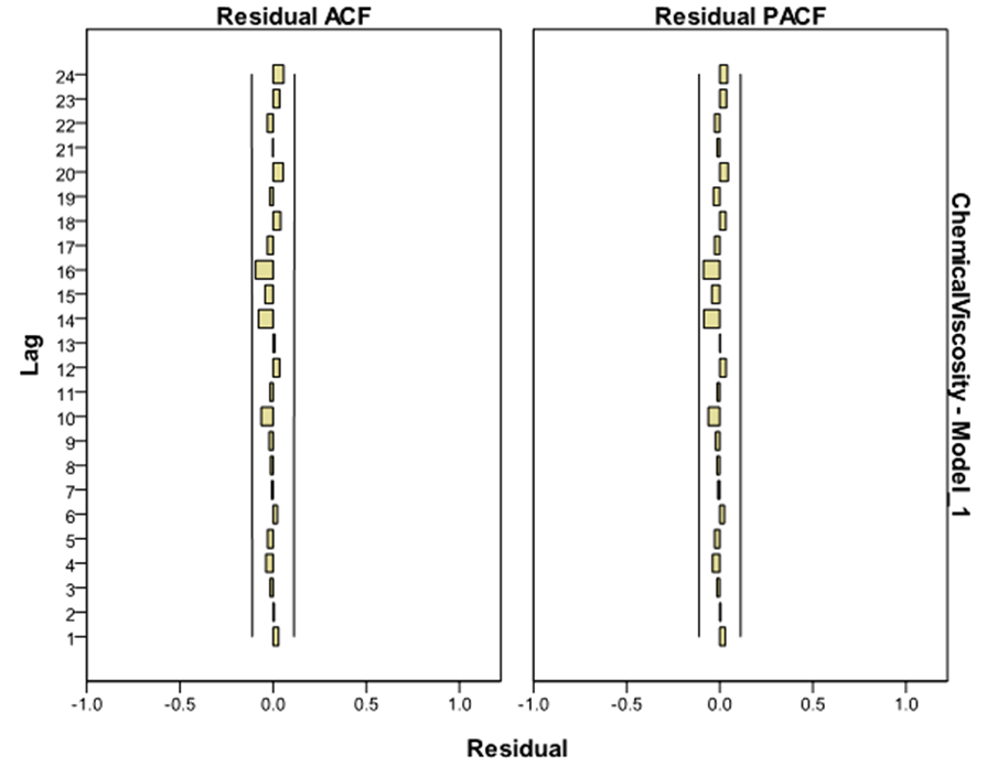 | Figure 6. Autocorrelation & Partial Autocorrelation Functions of the Residuals |
3.4. Forecasting with the Model
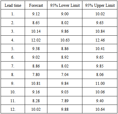
Forecasting based on the fitted model was computed up to lead time of 12, and the one-step forecasting and the 95% confidence limits are displayed in table 3.Table 3. One-step forecast of the ARIMA (1, 1, 1) Model
 |
| |
|
4. Summary
The sample acf and pacf of the original series (series D) were computed using the SPSS 17 Expert modeler and their graphs were plotted. These were used in identifying the appropriate model. The series exhibited non-stationary behaviour, following the inability of the sample acf of the series to die our rapidly even at high lags. The series was transformed by differencing once, and stationarity was attained. The plot of the differenced series indicated that the series is evenly distributed around the mean.Following the distribution of the acf and pacf of the differenced series, an ARIMA (1, 1, 1) model given by  was identified. The parameters of the fitted model were estimated. The model was then subjected to statistical diagnostic check using the Ljung-Box test statistic and the Normalized Bayesian Information Criterion (BIC). Analysis proved that the model is statistically significant, appropriate and adequate.The fitted model was used to forecast values of the chemical Viscosity Readings for a lead time
  of 12. The forecast is a good representation of the original data which neither decreases nor increases. The fitted model (ARIMA (1,1,1)) was compared with the two original models fitted to the same series by [4]. That is:AR (1) model given by:
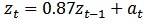 | (16) |
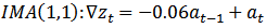
and IMA (1,1) model given by: 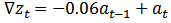 | (17) |
were fitted to the series D data. The Bayesian Information Criterion procedure was used in comparing these three models. That is: 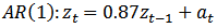 | (18) |
 | (19) |
And | (20) |
Analysis showed that the ARIMA (1, 1, 1) model is superior to the two other models having the least BIC value.The study aims at fitting a statistical time series model to the Chemical Viscosity Reading data. The data were extracted from [4] p. 529 called series D. The plots of the sample acf and pacf of the original series indicated that the series was not stationary. Transformation of the series was made by differencing to obtain stationarity. Following the distribution of the acf and pacf of the differenced series, an ARIMA (1, 1, 1) model was identified, the parameters of the model were estimated and diagnostically checked to prove its statistical significant and adequacy at both 0.05 and 0.01  –levels of significance under the Ljung-Box goodness of fit test. The Normalized Bayesian Information Criterion (BIC) was explored to confirm the adequacy of the model. Again, among a class of significantly adequate set of ARIMA (p,d,q) models of the same data set, the ARIMA (1,1,1) model was found as the most suitable model with least BIC value of –2.366, MAPE of 2.424, RMSE of 0.301 and R-square of 0.749. Estimation by Ljung-Box test with Q (18) = 9.746, 16 d.f and p-value of 0.880 showed no autocorrelation between residuals at different lag times. Finally, a forecast for a lead time (
 ) of 12 was made.
5. Conclusions
The ARIMA (1, 1, 1) model fitted to the Chemical Viscosity data is a better model than both the ARIMA (1, 0, 0) and ARIMA (0, 1, 1) models originally fitted to the same Series by Box-Jenkins in 1976. This showed that using the Bayesian Information Criterion procedure an improved or superior Box-Jenkins Models could be obtained.
References
| [1] | Makridakis, S., Wheelwright, S. C. and Hyndman, R. J. (1998): Forecasting Methods and Applications, John Wiley, New York. |
| [2] | Box, G. E. P., Jenkins, G. M. and Reinsel; G. C. (1994): Time Series Analysis; Forecasting and Control, Peason Education, Delhi. |
| [3] | Pankratz, A. (1983): Forecasting with Univariate Box-Jenkins Models: Concepts and Cases. John Wiley, New York. |
| [4] | Box, G. E. P., and Jenkins, G. M. (1976): Time Series Analysis; Forecasting and Control, Holden-Day Inc. U.S.A. |
| [5] | Enders, W. (2003): Applied Econometrics Time Series, John Wiley & Sons, U.S.A. |
| [6] | Ljung, G., and Box, G. E. P. (1978): On a Measure of lack of fit in Time Series Models. Biometrika 65:553-564 |
| [7] | Schwarz, G. E. (1978): Estimating the dimension of a Model. Annals of Statistics. 6(2): 461-464. |
| [8] | Akaike, H., (1977): On Entropy Maximization Principle In: Krishnaiah, P. R. (Editor). Application of Statistics, North-Holland, Amsterdam pp. 27- 41. |
| [9] | Priestley, M. B. (1981): Spectral Analysis and Time Series. Academic Press. London. |
 Abstract
 Reference
 Full-Text PDF
 Full-text HTML