Md Tanwir Akhtar, Athar Ali Khan
Department of Statistics and Operations Research, Aligarh Muslim University, Aligarh, 202002, India
Correspondence to: Md Tanwir Akhtar, Department of Statistics and Operations Research, Aligarh Muslim University, Aligarh, 202002, India.
| Email: |  |
Copyright © 2014 Scientific & Academic Publishing. All Rights Reserved.
Abstract
Log-logistic distribution is a very important reliability model as it fits well in many practical situations of reliability data analyses. Another important feature with the log-logistic distribution lies in its closed form expression for survival and hazard functions that makes it advantageous over log-normal distribution. It is therefore more convenient in handling censored data than the log-normal, while providing a good approximation to it except in the extreme tails. In this paper an attempt has been made to use Bayesian analytic and simulation methods for fitting the log-logistic reliability model. Real datasets are used for the purpose of illustrations. R code has been provided to implement in censored mechanism. Laplace approximation is implemented for approximating posterior densities of the parameters. Moreover, parallel simulation tools are also implemented with an extensive use of R.
Keywords:
Bayesian inference, Log-logistic distribution, Laplace Approximation, Simulation, Posterior density, R
Cite this paper: Md Tanwir Akhtar, Athar Ali Khan, Log-logistic Distribution as a Reliability Model: A Bayesian Analysis, American Journal of Mathematics and Statistics, Vol. 4 No. 3, 2014, pp. 162-170. doi: 10.5923/j.ajms.20140403.05.
1. Introduction
The model for which the Bayesian inference is desired is log-logistic distribution. This model is also used in reliability applications. It has the advantage (like the Weibull and exponential model) of having simple algebraic expressions for survival and hazard functions. It is therefore more convenient than the log-normal distribution in handling censored data, while providing a good approximation to it except in the extreme tails. Moreover, its relation with logistic distribution facilitates a lot in lifetime data analyses, that is, if lifetime  follows log-logistic distribution then logarithm of
  follows logistic distribution, which is a member of location-scale family of distributions. In many practical situations it has been seen that the non-Bayesian analysis of log-logistic distribution is not an easy task, whereas it can be a routine analysis when dealing in a Bayesian paradigm. Consequently, for the purpose of Bayesian analysis of log-logistic reliability model, two important techniques, that is, asymptotic approximation and simulation method are implemented using “Laplaces Demon” package of Statisticat LLC (2013). This package facilitates high-dimensional Bayesian inference, posing as its own intellect that is capable of impressive analysis, which is written entirely in R (R Core Team, 2013) environment and has a remarkable provision for user defined probability model (e.g., Akhtar and Khan, 2014). The function Laplace Approximation of Laplaces Demon package approximates the results asymptotically while the function Laplaces Demon simulates the results from posterior by using one of the several Metropolis algorithms of MCMC. These techniques are used both for intercept and regression models. Real datasets are used to illustrate the implementations in R. Censoring mechanism is also taken into account. Thus, Bayesian analysis of log-logistic distribution has been made with the following objectives:● To define a Bayesian model, that is, specification of likelihood and prior distribution.● To write down the R code for approximating posterior densities with Laplace approximation and simulation tools.● To illustrate numeric as well as graphic summaries of the posterior densities.
2. The Log-logistic Distribution
If  follows logistic distribution with location parameter
  and scale parameter
  having probability density function
 . Then the lifetime
  follows log-logistic distribution with scale parameter
  (> 0) and shape parameter
  (> 0) having probability density function of the form,
 | (1) |
where  and
and  . Corresponding reliability function and hazard function are, respectively,
 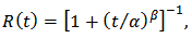 | (2) |
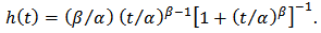 | (3) |
The mean of log-logistic distribution exists and is given by  only if
  . Because of its simple algebraic expression for the reliability and hazard functions, handling censored data is easier than with log-normal while providing a good approximation to it except in the extreme tails. The hazard function is identical to the Weibull hazard aside from the denominator factor
  . For
. For  , the hazard function is monotone decreasing. For
  , the hazard function resembles the log-normal as it increases from 0 to a maximum at
  , and then approaches 0 monotonically as
  (e.g., Lawless, 2003).
3. The Half-Cauchy Prior Distribution
The probability density function of half-Cauchy distribution with scale parameter  is given by
 The mean and variance of the half-Cauchy distribution do not exist, but its mode is equal to 0. The half-Cauchy distribution with scale
  is a recommended, default, non-informative prior distribution for a scale parameter. At this scale
  , the density of half-Cauchy is nearly flat but not completely (see Figure 1), prior distributions that are not completely flat provide enough information for the numerical approximation algorithm to continue to explore the target density, the posterior distribution. The inverse-gamma is often used as a non-informative prior distribution for scale parameter, however, this model creates problem for scale parameters near zero, Gelman and Hill (2007) recommend that, the uniform, or if more information is necessary the half-Cauchy is a better choice. Thus, in this paper, the half-Cauchy distribution with scale parameter
  is used as a non-informative prior distribution.
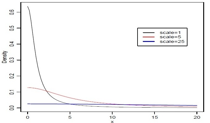 | Figure 1. It is evident from the above plot that for scale=25 the half-Cauchy distribution becomes almost uniform |
4. The Laplace Approximation
Many simple Bayesian analyses based on noninformative prior distribution give similar results to standard non-Bayesian approaches, for example, the posterior  -interval for the normal mean with unknown variance. The extent to which a noninformative prior distribution can be justified as an objective assumption depends on the amount of information available in the data; in the simple cases as the sample size
  increases, the influence of the prior distribution on posterior inference decreases. These ideas sometime referred to as asymptotic approximation theory because they refer to properties that hold in the limit as n becomes large. Thus, a remarkable method of asymptotic approximation is the Laplace approximation which accurately approximates the unimodal posterior moments and marginal posterior densities in many cases. In this section we introduce a brief, informal description of Laplace approximation method. Suppose
  is a smooth, bounded unimodal function, with a maximum at
  , and
, and  is a scalar. By Laplace's method (e.g., Tierney and Kadane, 1986), the integral
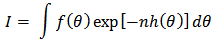 can be approximated by
 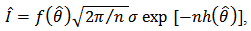 where
where As presented in Mosteller and Wallace (1964), Laplace's method is to expand about
  to obtain:
  Recalling that
  , we have
 Intuitively, if
  is very peaked about
  , then the integral can be well approximated by the behaviour of the integrand near
  . More formally, it can be shown that
 To calculate moments of posterior distributions, we need to evaluate expressions such as:
  , where
  (e.g., Tanner, 1996).
5. Fitting of Intercept Model
5.1. Fitting with Laplace Approximation
The Laplace approximation is a family of asymptotic techniques used to approximate integrals. It seems to accurately approximate unimodal posterior moments and marginal posterior densities in many cases. Here, for fitting of linear regression model we use the function Laplace Approximation which is an implementation of Laplace's approximations of the integrals involved in the Bayesian analysis of the parameters in the modelling pro- cess. This function deterministically maximizes the logarithm of the unnormalized joint posterior density using one of the several optimization techniques. The aim of Laplace approximation is to estimate posterior mode and variance of each parameter. For getting posterior modes of the log-posteriors, a number of optimization algorithms are implemented. This includes Levenberg-Marquardt (LM) algorithm which is default. However, we find that the Limited-Memory BFGS (L-BFGS) is a better alternative in Bayesian scenario. The limited-memory BFGS (Broyden- Fletcher-Goldfarb-Shanno) algorithm is a quasi-Newton optimization algorithm that compactly approximates the Hessian matrix. Rather than storing the dense Hessian matrix, L-BFGS stores only a few vectors that represent the approximation. It may be noted that Newton-Raphson is the last choice as it is very sensitive to the starting values, it creates problems when starting values are far from the targets, and calculating and inverting the Hessian matrix can be computationally expensive, although it is also implemented in Laplace Approximation. The main arguments of Laplace Approximation can be seen by using the function args as: 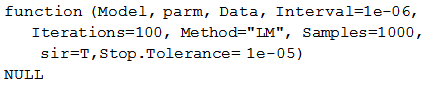 First argument Model defines the model to be implemented, which contains specification of likelihood and prior. Laplace Approximation passes two arguments to the model function, parm and Data, and receives five arguments from the model function: LP (the logarithm of the unnormalized joined posterior density), Dev (the deviance), Monitor (the monitored variables), yhat (the variables for the posterior predictive checks), and parm, the vector of parameters, which may be constrained in the model function. The argument parm requires a vector of initial values equal in length to the number of parameters, and Laplace Approximation will attempt to optimize these initial values for the parameters, where the optimized values are the posterior modes. The Data argument requires a listed data which must be include variable names and parameter names. The argument sir=TRUE stands for implementation of Sampling Importance Resampling algorithm, which is a bootstrap procedure to draw independent sample with replacement from the posterior sample with unequal sampling probabilities. Contrary to sir of LearnBayes package, here proposal density is multivariate normal not
  .
.
5.1.1. Roller Bearing Failure Time Data
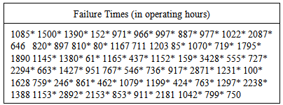
Let us introduce a lifetime dataset taken from Hamada et al. (2008) on page 110, so that all the concepts and computations will be discussed around that data. This dataset (see Table 1) comprises 11 observed failure times and 55 times when a test was suspended (censored) before item failure occurred  for a 4.5 roller bearing in a set of J-52 engines from EA-6B Prowler aircraft (Muller, 2003). Degradation of the 4.5 roller bearing in the J-52 engine has caused in-flight engine failures. The random variable is the time to failure T, and reliability is the probability that a roller bearing does not fail before time
  .
.Table 1. Roller bearing lifetime data for the Prowler attack aircraft
 |
| |
|
5.1.2. Data Creation
The function Laplace Approximation requires data that is specified in a list. For roller bearing failure time data the logarithm of failureTime will be the response variable. Since intercept is the only term in the model, a vector of 1’s is inserted into design matrix  . Thus,
  indicates only column of 1’s in the design matrix.
 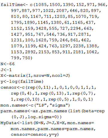 In this case, there are two parameters beta and log.sigma which must be specified in vector parm.name. The logposterior LP and sigma are included as monitored variables in vector mon.names. The number of observations is specified by
  , that is,
  . Censoring is also taken into account, where
  stands for censored and
  for uncensored values. Finally, all these things are combined in a listed form as MyData at the end of the command.
5.1.3. Initial Values
The function LaplaceApproximation requires a vector of initial values for the parameters. Each initial value is a starting point for the estimation of a parameter. Here, the first parameter, the beta has been set equal to zero, and the remaining parameter, log.sigma, has been set equal to log(1), which is zero. The order of the elements of the initial values must match the order of the parameters. Thus, define a vector of initial values  For initial values the function GIV (which stands for “Generate Initial Values”) may also be used to randomly generate initial values.
5.1.4. Model Specification
The function LaplaceApproximation can fit any Bayesian model for which likelihood and prior are specified. To use this method we must specify a model. Thus, for fitting of the roller bearing failure time data, consider that logarithm of failureTime follows a logistic distribution, which is often written as  and expectation vector
  is equal to the inner product of design matrix
  and parameter
  ,
, Prior probabilities are specified respectively for regression coefficient
  and scale parameter
  ,
,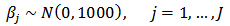
 The large variance and small precision indicate a lot of uncertainty of each
  , and is hence a weakly informative prior distribution. Similarly, half-Cauchy is a weakly informative prior for
  .
.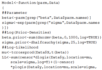
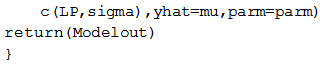
 In the beginning of the Model function contains two arguments, that is, parm and Data, where parm is for the set of parameters, and Data is the list of data. There are two parameters beta and sigma having priors beta.prior and sigma.prior, respectively. The object LL stands for loglikelihood and LP stands for logposterior. The function Model returns the object Modelout, which contains five objects in listed form that includes logposterior LP, deviance Dev, monitoring parameters Monitor, fitted values yhat and estimates of parameters parm.
5.1.5. Model Fitting
To fit the above specified model, the function LaplaceApproximation is used and its results are assigned to object Fit. Its summary of results are printed by the function print, which prints detailed summary of results and it is not possible to show here. However, its relevant parts are summarized in the next section.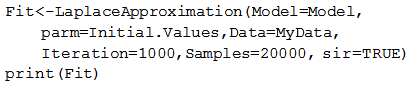
5.1.6. Summarizing Output
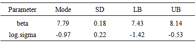
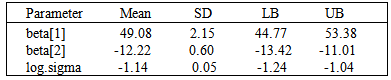
The function LaplaceApproximation approximates the posterior density of the fitted model, and posterior summaries can be seen in the following tables. Table 2 represents the analytic results using Laplace approximation method while Table 3 represents the simulated results using sampling importance resampling method.From these posterior summaries, it is obvious that, the posterior mode of intercept parameter  is
is  whereas posterior mode of
  is
is  . Both the parameters are statistically significant also. In a practical data analysis, intercept model is discussed merely as a beginning point. More meaningful model is simple regression model or multiple regression model which will be discussed in section 6. Simulation tool is being discussed in the next section.
Table 2. Summary of the asymptotic approximation using the function LaplaceApproximation. It may be noted that these summaries are based on asymptotic approximation, and hence Mode stands for posterior mode, SD for posterior standard deviation, and LB, UB are 2.5% and 97.5% quantiles, respectively
 |
| |
|
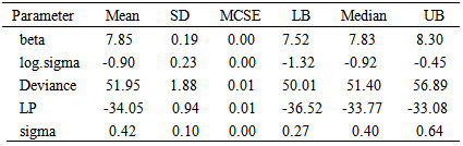
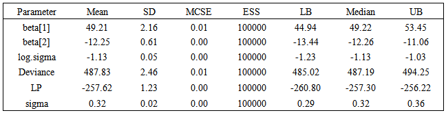
Table 3. Summary of the simulated results due to sampling importance resampling method using the same function, where Mean stands for posterior mean, SD for posterior standard deviation, MCSE for Monte Carlo standard error, ESS for effective sample size, and LB, Median, UB are 2.5%, 50%, 97.5% quantiles, respectively
 |
| |
|
5.2. Fitting with Laplaces Demon
In this section simulation method is applied to analyse the same data with the function Laplaces Demon, which is the main function of Laplace's Demon (Statisticat LLC, 2013). Given data, a model specification, and initial values, Laplaces Demon maximizes the logarithm of the unnormalized joint posterior density with Markov chain Monte Carlo (MCMC) algorithms, also called samplers, and provides samples of the marginal posterior distributions, deviance and other monitored variables. Laplace's Demon offers a large number of MCMC algorithms for numerical approximation. Popular families include Gibbs sampling, Metropolis-Hasting (MH), Random-Walk-Metropolis (RWM), slice sampling, Metropolis-within Gibbs (MWG), Adaptive-Metropolis-within-Gibbs (AMWG), and many others. However, details of MCMC algorithms are best explored online athttp://www.bayesian-inference.com/mcmc, as well as in the “LaplacesDemon Tutorial” vignette. The main arguments of the LaplacesDemon can be seen by using the function args as: 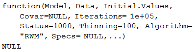 The arguments Model and Data specify the model to be implemented and list of data, which are specified in the previous section, respectively. Initial. Values requires a vector of initial values equal in length to the number of parameter. The argument Covar=NULL indicates that variance vector or covariance matrix has not been specified, so the algorithm will begin with its own estimates. Next two arguments Iterations=100000 and Status=1000 indicate that the Laplaces Demon function will update 10000 times before completion and status is reported after every 1000 iterations. The Thinning argument accepts integers between 1 and number of iterations, and indicates that every 100th iteration will be retained, while the others are discarded. Thinning is performed to reduced autocorrelation and the number of marginal posterior samples. Further, the Algorithm requires abbreviated name of the MCMC algorithm in quotes. In this case RWM is short for the Random-Walk-Metropolis. Finally, Specs=Null is default argument, and accepts a list of specifications for the MCMC algorithm declared in the Algorithm argument.
5.2.1. Initial Values
Laplace's Demon requires a vector of initial values for the parameters. Each initial value will be the starting point for an adaptive chain, or a non-adaptive Markov chain of a parameter. If all initial values are set to zero, then Laplace's Demon will attempt to optimize the initial values with the LaplaceApproximation function using a resilient backpropagation algorithm. So, it is better to use the last fitted object Fit with the function as.initial.values to get a vector of initial values from the LaplaceApproximation for fitting of LaplacesDemon. Initial values may be generated randomly with the GIV function. Thus, to obtain a vector of initial values the function as.initial.values is used as: 
5.2.2. Model Fitting
Laplace's Demon is stochastic, or involves pseudo-random numbers, its better to set a seed with set.seed function for pseudo-random number generation before fitting with LaplacesDemon, so results can be reproduced. Now, fit the prespecified model with the function LaplacesDemon, and its results are assigned to the object name FitDemon. Its summary of results are printed with the function print, and its relevant parts are summarized in the next section. 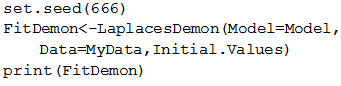
5.2.3. Summarizing Output
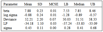
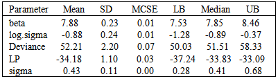
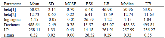
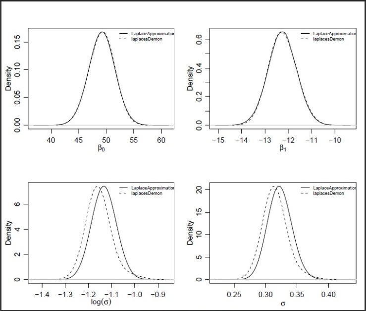
The LaplacesDemon simulates the data from the posterior density with Random-Walk-Metropolis and approximate the results which can be seen in the following tables. Table 4 represents the simulated results in a matrix form that summarizes the marginal posterior densities of the parameters over all samples which contains mean, standard deviation, MCSE (Monte Carlo Standard Error), ESS (Eective Sample Size), and 2.5%, 50%, 97.5% quantiles, and Table 5 summarizes the simulated results due to stationary samples. The complete picture of the results can also be seen in Figure 2.Table 4. Posterior summary of the simulated results due to all samples
 |
| |
|
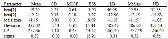
Table 5. Posterior summary of simulated results due to stationary samples
 |
| |
|
 | Figure 2. Plots of posterior densities of the parameters  and and  for the posterior distribution of log-logistic model using the functions Laplace Approximation and Laplaces Demon. It is evident from these plots that Laplace Approximation is excellent as it resembles with Laplaces Demon. The difference between the two seems magically for the posterior distribution of log-logistic model using the functions Laplace Approximation and Laplaces Demon. It is evident from these plots that Laplace Approximation is excellent as it resembles with Laplaces Demon. The difference between the two seems magically |
6. Fitting of Regression Model
6.1. Fitting with Laplace Approximation
6.1.1. Lifetimes of Steel Specimens Data
Kimber (1990) and Crowder (2000) discuss data on the times to failure of steel specimens subjected to cyclic stress loading of various amplitudes. The same data is discussed in Lawless (2003); they are for 20 specimens at each of the 14 stress amplitudes 32.0, 32.5, 33.0, ..., 38.0, 38.5. Failure times  are in numbers of thousands of stress cycles. None of the 280 times are censored. Figure 3 shows box plots of the log failure times at each stress amplitude. This suggests that log failure times tend to be smaller at higher amplitudes, and also that the dispersion decreases as the amplitude increases. Further exploratory data analysis suggests that a log-logistic distribution may provide a satisfactory description.
6.1.2. Data Creation
For fitting of lifetimes of steel specimens data with LaplaceApproximation, the logarithm of lifetime will be the response variable and stress level will be the regressor variable. Since an intercept term will be included, a vector of 1's is inserted into design matrix  . Thus,
  indicates that, there are two columns of independent variables, first column for intercept term and second column for regressor, in the design matrix.
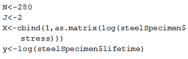
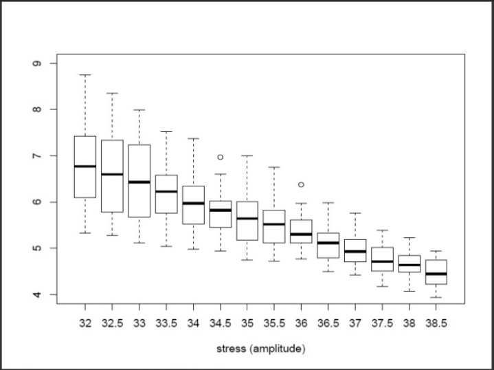 | Figure 3. Box plots of steel specimen log failure times at stress levels |
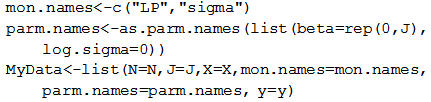 In this case of steel specimens data, all the three parameters including log.sigma are specified in a vector parm.names. The logposterior LP and sigma are included as monitored variables in a vector mon.names. Total number of observations is specified by
  , which is 280. Censoring is not included here. Finally, all these things are combined with object name MyData which returns the data in a list.
6.1.3. Initial Values
The initial value is taken as a starting point for the estimation of a parameter. So the first two parameters, the beta parameters have been set equal to zero, and log.sigma has been set equal to log(1), which is equal to zero. 
6.1.4. Model Specification
Fitting of the model with LaplaceApproximation, one must specify a model. For lifetimes of steel specimens data, consider that logarithm of lifetime follows logistic distribution. In this linear regression model with an intercept and one independent variable, the model may be specified as and expectation vector
  is an additive, linear function of vector of regression parameter
  , and design matrix
 Prior probabilities are specified respectively for regression coefficients,
  and scale parameter,
  ,
, It is obvious that all prior densities defined above are weakly informative. Thus, to specify above defined model create a function called Model as
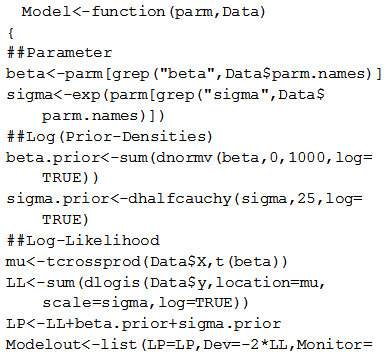
6.1.5. Model Fitting
Now, fit the above specified model using the function LaplaceApproximation by assigning the object name Fit, and its results are summarized in the next section.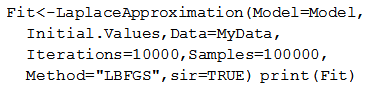
6.1.6. Summarizing Output
The relevant summary of results of the fitted regression model is reported in the following tables. Table 6 represents the analytic result using Laplace approximation method, and Table 7 represents the simulated results using sampling importance resampling method.Table 6. Posterior summary of the analytic approximation using the function Laplace Approximation, which is based on asymptotic approximation theory
 |
| |
|
Table 7. Posterior summary of the simulation due to sampling importance resampling method using the same function
 |
| |
|
6.2. Fitting with Laplace Demon
In this section, the function Laplaces Demon is used to analyze the same data, that is, Lifetimes of Steel Specimens. This function maximizes the logarithm of unnormalized joint posterior density with MCMC algorithms, and provides samples of the marginal posterior distributions, deviance and other monitored variables.
6.2.1. Model Fitting
For fitting the same model with the function LaplacesDemon by assigning the object name FitDemon, the R codes are as follows. Its summary of results is printed with the function print. 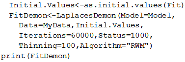
6.2.2. Summarizing Output
The function LaplacesDemon for the regression model, simulates the data from the posterior density with Random-Walk-Metropolis algorithm, and summaries of results are reported in the following tables. Table 8 represents the posterior summary of all samples, and Table 9 represents the posterior summary of stationary samples. The graphical summary of the results can be seen in Figure 4.Table 8. Posterior summary by the simulation method due to all samples using the function Laplaces Demon
 |
| |
|
Table 9. Posterior summary by the simulation method due to stationary samples using the same function
 |
| |
|
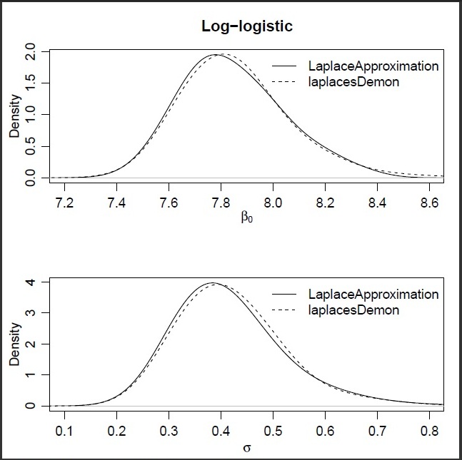
 | Figure 4. Plots of posterior densities of the parameters  , ,  , ,  and and  of log-logistic model using the two different methods, that is, asymptotic approximation and simulation methods of log-logistic model using the two different methods, that is, asymptotic approximation and simulation methods |
7. Discussion and Conclusions
In this article, Bayesian approach is applied to model the real reliability data using log-logistic distribution. Two important techniques, that is, asymptotic approximation and simulation method are implemented using the functions of “Laplaces Demon” package of Statisticat LLC. The main body of the manuscript contains the complete description of R code both for intercept and regression models of log-logistic distribution. The function Laplace Approximaion approximates the results asymptotically and simulation is made by the function Laplaces Demon. Results of these two methods are very close to each other. The excellency of these approximations seem clear in the plots of posterior densities. It is evident from the summaries of results that the Bayesian approach based on weakly informative priors is simpler to implement than the classical approach. The wealth of information provided in these numeric and graphic summaries are not possible in classical framework (e.g., Lawless, 2003). On the other hand, it is quite simple in Bayesian paradigm using tools like R. Furthermore, this approach can also be used for multiple regression models, and can be extended for hierarchical modelling relevant in reliability. Software developed in this paper can also be applied for Bayesian survival analysis.
References
| [1] | Akhtar, M. T. and Khan, A. A. (2014). Bayesian analysis of generalized log-Burr family with R. SpringerPlus 2014 3:185. |
| [2] | Crowder, M. J. (2000). Tests for a family of survival models based on extremes. In Recent Advances In Reliability Theory, N. Limnios and M. Nikulin, Eds., pp. 307-321. Birkhauser, Boston. |
| [3] | Gelman, A. and Hill, J. (2007). Data Analysis Using Regression and Multilevel/Hierarchical Models. Cambridge University Press, New York. |
| [4] | Hamada, M. S., Wilson, A. G., Reese, C. S., and Martz, H. F. (2008). Bayesian Reliability. Springer, New York. |
| [5] | Kalbfleisch, J. D. and Prentice, R. L. (2002). The Statistical Analysis of Failure Time Data. Second Edition. John Wiley & Sons, Inc., Hoboken, New Jersey. |
| [6] | Kimber, A. C. (1990). Exploratory data analysis for possibly censored data from skewed distributions. Appl. Stat., 39, 21-30. |
| [7] | Lawless, J. F. (2003). Statistical Models and Methods for Lifetime Data. Second Edition. John Wiley & Sons, Inc., Hoboken, New Jersey. |
| [8] | Mosteller, F. and Wallace, D. L. (1964). Inference and Disputed Authorship: The Federalist. Reading: Addison- Wesley. |
| [9] | Muller, C. (2003). Reliability analysis of the 4.5 roller bearing. Master’s thesis, Naval Postgraduate School. |
| [10] | Nelson, W. B. (I972). Graphical analysis of accelerated life test data with the Inverse power law model, IEEE Trans. Reliab., R-21, 2-11. |
| [11] | R Core Team (2013). R: A language and environment for statistical computing. R Foundation for Statistical Computing, Vienna, Austria. URL http://www.R-project.org/. |
| [12] | Schmee, J. and Nelson, W. (1977). Estimates and approximate confidence limits for (log) normal life distributions from singly censored samples by maximum likelihood. General Electric C. R. & D. TIS Report 76CRD250. Schenectady, New York. |
| [13] | Statisticat LLC (2013). LaplacesDemon: Complete environment for Bayesian inference. R package version 13.09.01, URL http://www.bayesian-inference.com/software. |
| [14] | Tableman, M. and Kim, J. S. (2004). Survival Analysis Using S: Analysis of Time-to-Event Data. Chapman & Hall/CRC, Boca Raton. |
| [15] | Tanner, M. A. (1996). Tools for Statistical Inference. Springer-Verlag, New York. |
| [16] | Tierney, L. and Kadane, J. B. (1986). Accurate approximations for posterior moments and marginal densities. Journal of the American Statistical Association 81, 82-86. |
 Abstract
 Reference
 Full-Text PDF
 Full-text HTML