| [1] | Al-Joboori, A.N., (2002), "On Shrunken Estimators for the Parameters of Simple Linear Regression Model", Ibn-Al-Haitham J. for Pure and Applied Sciences, 15,(4A), 60-67. |
| [2] | Al-Joboori, A.N., (2010), "Pre-Test Single and Double Stage Shrunken Estimators for the Mean of Normal Distribution with Known Variance", Baghdad Journal for Science, 7, 4, 1432-1442. |
| [3] | Al-Joboori, A.N., Khalaf, B.A. and Hamza, S., (2010)," Estimate the Scale Parameter of Exponential Distribution Via Modified Two Stage Shrinkage Technique", Journal College of Education, 6, 62-75. |
| [4] | Al-Juboori, A.N. (2011), "On Significance Testimator for the Shape Parameter of Generalized Rayleigh Distribution ". Journal of AL-Qadisyia. 3, 2, 390-399. |
| [5] | Al-Juboori, A.N. (2012), "Estimate the Reliability Function of Exponential Distribution Via Pre-Test Single Stage Shrinkage Estimator". Accepted to publish, Tikrit of Mathematics and Computer Journal. |
| [6] | Askoy, H. (2000), “Use of gamma distribution in hydrological analysis”, Turkish Journal of Engineering and Environmental Science, 24, 419-428. |
| [7] | Birnbaum, Z. W. and S. C. Saunders (1958), “A statistical model for life lengths of materials”, Journal of the American Statistical Association, 53, 153-160. |
| [8] | Bhunya, P. K., R. Berndtsson, C. S. P. Ojha and S. K. Mishra (2007), “Suitability of gamma, chi-square, Weibull, and beta distributions as synthetic unit hydrographs”, Journal of Hydrology, 334, 28-38. |
| [9] | Drenick, R. F. (1960), “Mathematical aspects of the reliability problem”, Journal of the Society for Industrial and Applied Mathematics, 8, 125-149. |
| [10] | Gupta, S. S. and P. A. Groll (1961), “Gamma distribution in acceptance sampling based on life tests”, Journal of the American Statistical Association, 56, 942–970. |
| [11] | Herd, G. R. (1959), “Some statistical concepts and techniques for reliability analyses and prediction”, Proceedings from Fifth National Symposium on Reliability Control, Philadelphia PA, 126-136. |
| [12] | Jensen, J., I. Batina, R. C. Hendriks and R. Heusdens (2005), “A study of the distribution of time-domain speech samples and discrete Fourier coefficients”, Proceedings of SPS-DARTS 2005 (The first annual IEEE BENELUX/DSP Valley Signal Processing Symposium), 155-158. |
| [13] | Keaton, M. (1995), “Using the gamma distribution to model demand when lead time is random”, Journal of Business Logistics, 16, 107-131 |
| [14] | Kim, C. and R. M. Stern (2008), “Robust signal-to-noise ratio estimation based on waveform amplitude distribution analysis”, Proceedings of the Interspeech 2008 Conference, Brisbane, Australia, 2598-2601. |
| [15] | Martin, R. (2002), “Speech enhancement using mmse short time spectral estimation with gamma distributed speech priors”, in Proceedings of the IEEE International Conference on Acoustics, Speech, Signal Processing, I, Orlando FL, 253–256. |
| [16] | Pearson, K. (1895), “Contributions to the mathematical theory of evolution.-II. Skew variation in homogeneous material”, Philosophical Transactions of the Royal Society of London, A, 186, 343-414. |
| [17] | Segal, M. R., H. Salamon and P. M. Small (2000), “Comparing DNA fingerprints of infectious organisms", Statistical Science, 15, 27-45. |
| [18] | Simpson, J. (1972), “Use of the gamma distribution in single-cloud rainfall analysis”, Monthly Weather Review, 100, 309-312. |
| [19] | Thompson,J.R., (1968), "Some Shrinkage Techniques for Estimating the Mean", J. Amer. Statist. Assoc, 63, 113-122. |
| [20] | Wein, L. M. and M. Baveja (2005), “Using fingerprint image quality to improve the identification performance of the U.S. visitor and immigrant status indicator technology program”, Proceedings of the National Academy of Sciences, 102, 7772-7775. |
 Abstract
 Reference
 Full-Text PDF
 Full-text HTML
 that is based upon the result of a test of the hypothesis H0: θ = θ0 against the hypothesis HA: θ ≠ θ0 with level of significance
  . If H0 is accepted we used
  , where the weighting factor
  is a function of the test statistic for testing H0 or may be constant such that
  . However if H0 is rejected we used
  , where
  and
and  is the classical estimator of θ (MLE or MVUE). Choosing the weighting factor
  , (i =1,2) appropriately, an expression for the Mean Squared Error (MSE) and Bias Ratio [B(.)] of
  were derived and comparisons were made with classical estimator (
 ) in the sense of efficiency and with some related earlier studies.


 and suitable region R and create comparisons of the numerical results with
  and with some existing studies.A numerical study is carried out to appraise these effects of proposed estimators.Shrinkage technique was introduced by Thompson [19] as follows
 , represents a shrinkage weight factor specifying the degree of belief in
  and 1-
 specifying the degree of belief in θ0 . We used the form (1.4) above to estimate the scale parameter θ of Gamma distribution in case
  is chosen as follows:-
 and
and  is the classical estimator of θ (MLE or MVUE), then the estimator which is defined in (1.4) will be written as below
 , i = 1,2;
  represents as shrinkage weight factors which may be a functions of
  or may be constants. The resulting estimator (1.6) is known as preliminary test single stage shrinkage estimator (PTSSSE).Several authors had studied the estimator defined in (1.6) for special distribution for different parameters and suitable regions (R) as well as for estimate the parameters of linear regression model. For example see [1], [2], [3], [4], [5] and [19].
 and shape parameter α .i.e. ;
  ∼ G(α,θ) for i=1,2,3,...n.And assume that the shape parameters
  is known ( say α =
  )The maximum likelihood function L (ti;
  ,
, ) is defined as below : -

 ,
, ) is:-
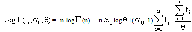
 with respect to (w.r.t)
  is as below:-
 as below
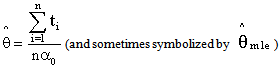
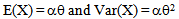
 ∼ Gamma (nα0,θ/nα0) .It is easy of note that
  is unbiased estimator.i.e.; E (
 ) = θ and MSE (
 ) = Var (
 ) = θ2/nα0.
  for estimate the scale parameter θ of Gamma distribution when a prior information θ0 available about θ with known shape parameter
  as below:-
 = 0 and
  = k in equations (1.5).And the region R which is defined in (1.5) will be as below:
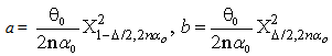
 and
and  are respectively the lower and upper 100(
 /2) percentile point of Chi-square distribution with (2nαo) degree of freedom.The expressions for Bias of the estimator
  is as follows:-
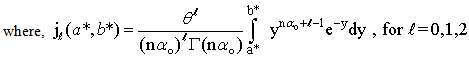
 where
where  is the complement region of R in real space and
  is a (PDF) of
  which has the following forms
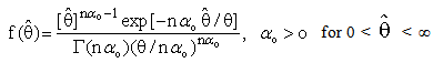


 ) of the estimator
  is defined below
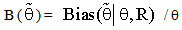
 is given as below:


 w.r.t. the classical estimator (
 ) is defined as below:-
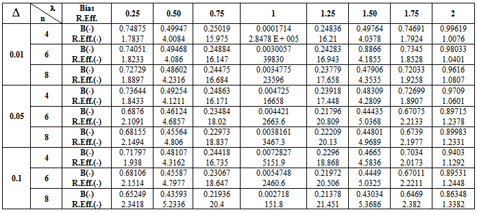
 . These computations (using Mat. LAB programs) were performed for
  = 0.01, 0.05, 0.1, λ = 0.25(0.25)2 and n = 4,6,8.These computations are given in three annexed tables. The observation mentioned in the tables lead to the following results:1. R.Eff (
 ) were adversely proportional with small value of α0 and n specially when θ0 close to θ.2. R.Eff (
 ) are maximum when θ = θ0(λ = 1) for all
  , α0 and n. This feature shown the important usefulness of prior knowledge which given higher effects of proposed estimator as well as the important role of shrinkage technique and its philosophy.3. Bias Ratio [B (
 )]
)] were reasonably small when θ
  θ0, otherwise start to be maximum for all
  and n. This property shown that the proposed estimator
  is very closely to unbiased ness especially when θ
  θ0.4. Bias Ratio [B (
 )] were at most decreasing function with
  for all n and λ.5. Effective Interval [the values of λ that makes R. Eff. greater than one] for
  was [0.25, 2] for all α0, n and
  . Here the pretest criterion is very important for guarantee that prior information is very closely to the actual value and prevent it faraway from it, which get optimal effect of the considered estimator to obtain high efficiency.6. The suggested estimator
  is more efficient than the classical estimator
  specially when θ0 is very close to θ which is given the effective of
  when given an important weight of prior knowledge. And the augmentation of efficiency may be reach to tens times. Also
  more efficient than the estimator introduced by [19] in the sense of Mean Squared Error and Relative Efficiency.7. When the shape parameter of Gamma distribution equal to one [α0 = 1], the distribution become an Exponential distribution, thus the suggested estimator
  in this case is more efficient than the estimator introduced by [3].
  when α0 = 1
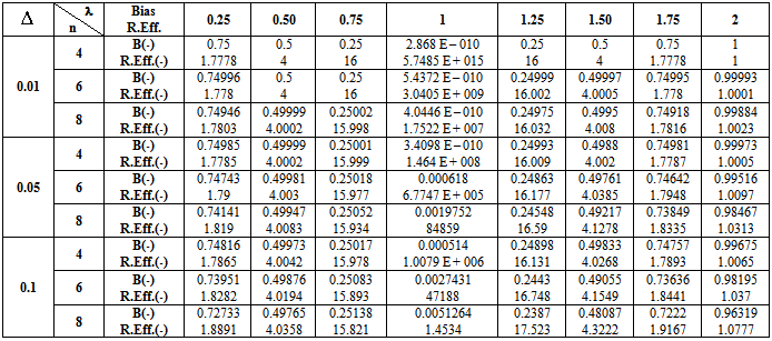
 when α0 = 2
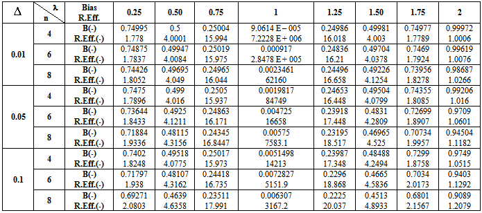
 when α0 = 3