Sachin Kumar1, Anil Kumar1, Rakesh Kumar2, J. K. Pathak3, Mohd. Alam4
1Department of Physics, Hindu college, Moradabad, 244001, India
2Department of Mathematics, Hindu college, Moradabad, 244001, India
3Department of Zoology, Hindu College, Moradabad, 244001, India
4WWF-India, Ramganga Mitra, Ramganga Vihar, Moradabad
Correspondence to: Sachin Kumar, Department of Physics, Hindu college, Moradabad, 244001, India.
| Email: |  |
Copyright © 2014 Scientific & Academic Publishing. All Rights Reserved.
Abstract
Excess of biochemical oxygen demand (BOD) is the most outstanding danger at present for survival of living being in the surface water. In this paper, we analyse the BOD of surface water using wavelet analysis. Wavelet analysis is a new mathematical tool developed in last two decade. Wavelets have special ability to examine signals or data sets simultaneously in both time and frequency scale. Consequently, we get hidden information of signal in a new plane which is called time frequency plane. In the present manuscript we interpret the data of BOD of river Ramganga by wavelet method. We used ‘db8’ wavelet of Daubechies wavelet family. The data of BOD is taken during the period from Jun 2005 to May 2008.
Keywords:
Daubechies wavelet, River ramganga, Time frequency plane, Wavelet analysis
Cite this paper: Sachin Kumar, Anil Kumar, Rakesh Kumar, J. K. Pathak, Mohd. Alam, Spectral Analysis of Biochemical Oxygen Demand in River Water: An Analytical Approach of Discrete Wavelet Transform, American Journal of Mathematics and Statistics, Vol. 4 No. 2, 2014, pp. 107-112. doi: 10.5923/j.ajms.20140402.06.
1. Introduction
To conserve and manage lotic water resources efficiently is very critical. A holistic approach should be adopted for proper management of the aquatic resources especially running water. As a result of anthropogenic activities along the river bed results degradation of water quality and ultimately affects the aquatic ecosystem. The physical, chemical and biological components of the aquatic system should be monitored at regular basis to understand their function and relationship. Due to economic activity in river Ramganga flood plain. The water get polluted. Water quality indicators consists of physical, chemical and biological variables designed to provide clear signals about the status and changes of the system (Alegue and Gnauck, 2006) [1]. Some of the variables such as biochemical oxygen demand (BOD) act as stressor. Signal analysis method enable the extraction of information projecting in the time frequency and time scale domains (Mallat, 1998) [2]. Using discrete wavelet transformation method of Daubechies wavelet family [3, 4] in studying the variations, the structural characteristics of BOD at different time scale reveals information necessary in the diagnosing of water quality pollution and selecting an appropriate management strategy for pollution control.In India a number of studies have been made to describe the hydrochemistry of several stream and rivers. Kulwinder Singh Parmar et al. (2012) [5] studied the water quality parameters by using Daubechies wavelet (db5). Also the impacts of hydrological conditions of the water on biological community of the water body have been documented (Pathak, 2008) [6]. In India as a developing country, industrial pollution is one of the main causes of water pollution has been investigated in several major rivers. The necessity to efficiently conserve and manage freshwater resources is becoming more and more urgent. This is as a result of growing world population and economic activities with the subsequent degradation of freshwater resources as a result of anthropogenic pollution. To sustainable management of freshwater ecosystems an understanding of the basic physical, chemical and biological components, their functions and interrelationship is necessary. Wavelet is a new tool in the emerging field of data analysis for Physicists, Engineers Mathematicians and environmentalists [7, 8, 9]. It represents an efficient computational algorithm under the interest of a broad community. Fourier sine’s extracts only frequency information from a time signal, thus losing time information, while wavelet extracts both time evolution and frequency composition of a signal.
2. Methodology
Wavelet analysis allows to isolate and manipulate specific types of patterns hidden in masses of data. Alfred Haar, a Hungarian Mathematician was the first who introduced some functions in 1909. These functions are Haar wavelets. From time to time over the next several decades, other precursors of wavelet theory arose. In 1987 Ingrid Daubechies discovered a whole new class of wavelets which is known as ‘Daubechies Wavelets’. The Daubechies wavelets turn the theory into a practical tool that can be easily programed and used with a minimum of mathematical training.
2.1. Discrete Wavelet Transform (DWT) and Multiresolution Analysis (MRA)
Wavelets are a special kind of functions which exhibits oscillatory behavior for a short period of time and then die out. For any two real numbers a and b, a wavelet function is defined as: | (1) |
where a is scaling parameter which gives the dilate or compressed version of wavelet function.And b is a parameter gives a translated version of wavelet function called translation parameter. If we choose  and
and  , we get discrete wavelet
 | (2) |
The wavelet transform of a signal captures the localized time frequency information of the signal. A multi resolution analysis (MRA) is a radically new recursive method for performing discrete wavelet analysis. A MRA for  introduced by Mallat [10, 11] and extended by other researchers [12, 13, 14, 15] consists of a Sequence
  of closed subspaces of
  , a space of square integrable functions, satisfying following properties;1.
  2.
2.  3. For every
  ,
,  4. There exists a function
  such that
  is orthonormal basis of
  .The function
  is called the scaling function of the given MRA and property 3 implies a dilation equation
 where
where  is a low pass filter and defined as
 Now consider
  be the orthogonal compliment of
  in
in  i.e.,
i.e.,  | (3) |
If  be any function then
  where
where  are high pass filters.We can express a signal in terms of bases of
  space and
  space. If we combine the bases of
  and
and  space, we can express any signal in
  space.Using the same argument, we can write
 In general
 But
But  Therefore
 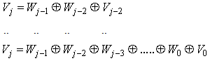 | (4) |
Let  be a function sampled at regular time interval
  , where
  is an integer . S is split into a “blurred” version a1 at the coarser interval
  and “detail” d1 at scale
  . This process is repeated and gives a sequence S, a1, a2, a3, a4,…..of more and more blurred versions together with the details d1, d2, d3, …….removed at every scale (
 in am and dm-1). Here am’S and dm’S are approximation and details of original signal. After N iteration S can be reconstructed as S=aN+d1+d2+d3+d4+d5 +…+dN. The approximations are the high-scale, low-frequency components of the signal. The details are the low-scale, high-frequency components. Thus the original signal, S, passes through two complementary filters in which one is low pass filter and second one is high pass filter.
2.2. Daubechies Wavelet 8
The Daubechies wavelets are compactly supported orthogonal wavelets. The Daubechies family is named after Ingrid Daubechies who invented the compactly supported orthonormal wavelet, making wavelet analysis in discrete time possible. The order of the Daubechies functions denotes the number of vanishing moments. Higher order Daubechies functions are not easy to describe with an analytical expression. A vanishing moment limits the wavelet's ability to represent polynomial behavior or information in a signal. The wavelet and scaling functions for the Daubechies functions with order 8 are shown in figure 1 and figure 2.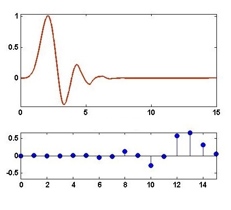 | Figure 1. Scaling function (upper) and decomposition low pass filter (lower) of Daubechies wavelet of order 8 (“db8”) |
 | Figure 2. Wavelet function (upper) and decomposition high pass filter (lower) of Daubechies wavelet of order 8 (“db8”) |
3. Study Area
River Ramganga, is the most important tributary of holy river Ganga, is spring fed originated from the southern slopes of Dudhatoli (3,110 masl) of middle Himalaya of Uttrakhand state. The river enters the plains at Kalagarh where a famous hydroelectric earthen dam has been constructed in 1975. The river traverses near about 158 km before it meets the reservoir and continues to downstream for about 370 km before joining river Ganga at Kannauj of Uttar Pradesh state. The study area of the river catchment lies between north latitude 29°29’42” and 28°49’32” and east longitude 78°45’37” and 78°47’53. The river navigates through varied catchments covered with forestland, agriculture field and human settlements with various types of industrial setups. The catchment area in downstream is inhabited on alluvial deposits of Quartz energy period. The alluvial deposits has been drained and transported from the Himalayas ranges by the Ganga river system and specially the river Ramganga. In order to carry out in depth investigation, nine sampling stations at different segments of river Ramganga were selected on the basis of varied topographical conditions, agricultural, social pattern and on the locations of various large and small-scale industries and also on the basis of human settlement. | Table 1. Sampling Spots in downstream river Ramganga |
| | 1 | SS1 | Kalagargh | | 2 | SS2 | Bhutpuri | | 3 | SS3 | Seohara | | 4 | SS4 | Mishripur | | 5 | SS5 | Agwanpur | | 6 | SS6 | Jigar colony | | 7 | SS7 | Lalbhagah | | 8 | SS8 | Jamamasjid | | 9 | SS9 | Kathgargh |
|
|
4. Result and Discussion
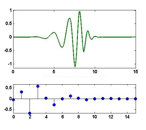
In order to perform a more detailed investigation we decompose the time series of BOD at different scale by using discrete wavelet transform. The original time series of BOD is shown in figure 3. A full decomposition of BOD time series is shown in figure 4(a) and figure 4(b). In decomposition, figures a1, a2, a3, a4, a5, a6, a7 and a8 are approximations and d1, d2, d3, d4, d5, d6, d7, and d8 are details of the of BOD time series at different time mode. | Figure 3. Wavelet decomposition of BOD time series. Original time series s and its approximations |
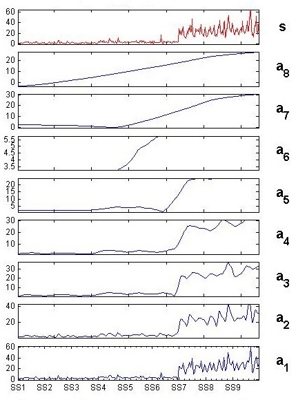 | Figure 4(a). Wavelet decomposition of BOD time series. Original time series s and its approximations |
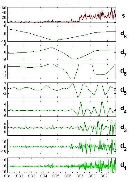 | Figure 4(b). Wavelet decomposition of BOD time series. Original time series s and its details |
Original signal S is taken as monthly interval. Approximation a1 represents the bi-monthly behavior of the signal S, a2 represents quarterly behavior of the signal, a3 is bi-quarterly or 8-months mode behavior, a4 is the behavior of signal in 16-months mode and so on. Likewise details d1 exhibits monthly variation, d2 shows bi-monthly variation and d3 is quarterly variation in the value of BOD also d4, d5, d6, d7 and d8 are variation in the value of BOD in 8, 16, 32, 64, and 128 months mode, respectively. A peak in a detail shows rapid fall or rise in the value of BOD in that time mode. The measurement of BOD depends on anthropogenic driving forces. Fluctuation in downstream over time may be as a result of effluent load (Fig. 4(b)).In signal analysis, the low-frequency content of the signal is an important part. Because it gives the identity of the signal. Trend is the slowest part of the signal means lowest frequency part of the signal. In wavelet analysis terms, this is correspond to the greatest scale value. In figure 4(a) it is corresponds to a8. As the scale increases, the resolution decreases, producing a better estimate of the unknown trend. A trend of the BOD signal is exhibits in figure 5. It is clear that the value of BOD level is lie between 0-30 ppm during the time period from 2005 to 2008.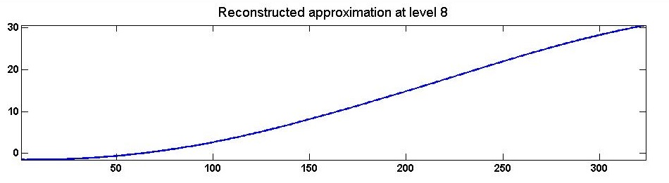 | Figure 5. Trend of BOD in downstream of river Rāmgangā |
Figure 6 depicts the histograms for Approximation a5. A cumulative histogram is a mapping that counts the cumulative number of observations in all of the bins up to the specified bin. The histogram provides important information about the shape of a distribution. A variance in the value of BOD during three years in individual sampling spot is clearly depicts in approximation a5 of the decomposition. It is clear that the BOD level is minimum in Sampling spots Kalagargh, Bhutpuri, Seohara, Mishripur, Awganpur, varied between 3-10 ppm, while in sampling spots Jamamasjid and Kathgargh shows maximum BOD level. 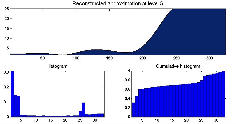 | Figure 6. Approximation a5 (upper) and its histogram and cumulative histogram (lower) |
Histogram of approximation a5 shows that 60 percent water of river is below the prescribe limit of BOD by WHO and Indian Standards. In other words, 40 percent of river segment is highly polluted. A comparative statistics of BOD time series in different time modes is shown in Table 2 and Table 3.| Table 2. Statistical analysis of BOD time series at different time mode |
| | S. N. | Time mode | level | Mean | Median | Mode | Standard deviation | | 1 | Monthly | S | 10.66 | 3.84 | 3.40 | 12.48 | | 2 | Bi-monthly | a1 | 10.67 | 3.78 | 2.76 | 12.04 | | 3 | Quarterly | a2 | 10.67 | 3.79 | 2.66 | 11.47 | | 4 | Bi-quarterly | a3 | 10.64 | 4.04 | 1.82 | 11.09 | | 5 | 16-months mode | a4 | 10.66 | 3.93 | 2.05 | 11.04 | | 6 | 32-months mode | a5 | 10.69 | 3.93 | 2.04 | 10.93 | | 7 | 64-months mode | a6 | 10.81 | 3.04 | 2.29 | 10.95 | | 8 | 128-months mode | a7 | 10.79 | 3.92 | 2.03 | 10.93 | | 9 | 256-months mode | a8 | 11.47 | 9.74 | 1.01 | 10.59 |
|
|
| Table 3. Statistical analysis of variation in BOD time series at different time mode |
| | S.N. | Time mode | level | Max | Min | Mode | | 1 | Monthly variation | d1 | 16.34 | -14.88 | 0.191 | | 2 | Bi-monthly variation | d2 | 14.46 | -18.75 | -0.483 | | 3 | Quarterly variation | d3 | 8.36 | -8.75 | 0.098 | | 4 | Bi-quarterlyvariation | d4 | 5.96 | -5.88 | 0.240 | | 5 | 16-months mode variation | d5 | 6.42 | -5.36 | 0.341 | | 6 | 32-months mode variation | d6 | 4.89 | -3.74 | 0.147 | | 7 | 64-months mode variation | d7 | 1.32 | -0.91 | 0.019 | | 8 | 128-months mode variation | d8 | 4.32 | -5.94 | -5.769 |
|
|
Table 2 explains the statistic of original time series and its approximations in different time mode. A high value of standard deviation indicates that the data points are spread out in a wide range. Because of high standard deviation, data is spread widely in all time mode. Table 3 tells about the amplitude of the change. Large value of amplitude indicates that there is a rapid change in the value of BOD in that time interval. According to Table 3, details d1 and d2 have a large Maximum of 16.34, 14.46) and Minimum of -14.88, -18.75. It reveals that monthly and bi-monthly variation is relatively high. A frequency distribution of the variation in the value of BOD is shown in fig.7. It is clear from the frequency distribution that the sharp variations have a small contribution as compared with the low variations at all scale. From the analysis presented above we note that the monthly and bi- monthly variation in the value of BOD of river Ramganga is relatively high. Which is supported by the decomposition of time series mode as presented in figure 4b and Table 3. However, we note that the anthropogenic activity has play an important role in increasing BOD level in the water system in this parameter.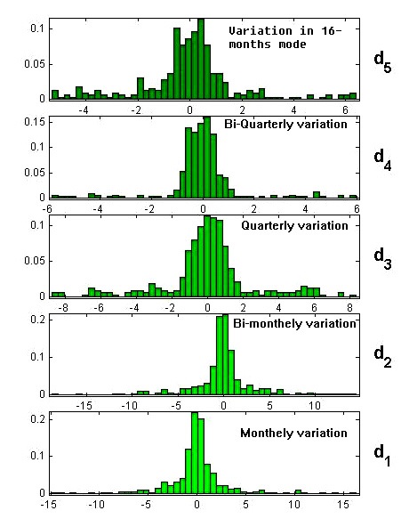 | Figure 7. Frequency distribution of variation in BOD time series at different scale |
5. Conclusions
Signal analysis of BOD a stressor indicator by Daubechies wavelet (db 8 level 8) make it possible to quantify the variations on a particular time frame and variations and interrelationships existing between natural and anthropogenic interferences of water quality indicators. The wavelet method allows the decomposition of signal according to different frequency levels which characterize the intensity of natural and man-made disturbances.A histogram is a graphical representation showing a visual impression of the distribution of data. According to the behaviour studied, it is possible to conjecture that the difference between all-time series can be directly associated with the large number of anthropogenic activity. Taking into account these results we have shown, the wavelet analytical approach provides a simple and accurate framework for modelling the statistical behaviour of BOD turbulence.
ACKNOWLEDGEMENTS
Financial support by University Grant Commission, New Delhi to Sachin Kumar for conducting research work on wavelet is greatly acknowledged. The author (J. K. Pathak) is grateful to DST, government of India for providing financial support to carryout river basin study.
References
| [1] | Jean Duclos Alegue, Albrecht Gnauck, 2006. Signal Analysis of Water Quality Indicators. Enviro. Info 2006 (Graz). Managing Environmental Knowledge, 369-376. |
| [2] | Mallat,S. ,1998. A wavelet Your of Signal Processing. Academic Press, New York. |
| [3] | Daubechies, I., 1992. Ten lectures on wavelets, CBS-NSF, Regional Conference in Applied Mathematics, SIAM Philadelphia 61, 278-285. |
| [4] | Daubechies, I. Sep. 1990, The wavelet transform, time frequency localization and signal analysis, IEEE Trans. Inform. Theory, 36, 961-1005. |
| [5] | Parmar Kulwinder Singh, 2012, Bhardwaj Rashmi. Analysis of Water Parameters Using Daubechies Wavelet, American Journal of Mathematics and Statistics, 2(3): 57-63. |
| [6] | Pathak. J. K., 2008, Evaluation of limnological characteristics and its trophic status of river Ramganga of western Uttar Pradesh. FTR submitted to DST, Government of India. |
| [7] | Antoine. J. P., 2004, Wavelet analysis: A new tool in Physics, Wavelets in Physics, Van Der Berg, J. C., ed., 9-21. |
| [8] | Bonami. A., Soria. F. and Weiss. G., 1993, Band limited wavelets, J. of Geometric analysis, 3, 544-578. |
| [9] | Chui. C. K., 1992, An introduction to wavelets, Academic Press, New York. |
| [10] | Mallat, S. G., 1989, “Multiresolution Approximations and Wavelet Orthonormal Bases of” Trans. Amer. Math. Soc., 315, pp. 69-87. |
| [11] | Mallat, S. G., 1989, “A Theory for Multiresolution Signal Decomposition, The Wavelet Representation,” IEEE Trans. On Pattern Analysis and Machine Intelligence, 11, pp. 674-693. |
| [12] | Cohen. A., Daubechies. I., and Vail. P., 1993, Wavelets on the interval and fast algorithms, Journal of Applied and Computational Harmonic Analysis, 1, 54-81. |
| [13] | Coifman. R. R., and Wickerhauser. M. V., March 1992, Entropy based algorithms for best basis selection, IEEE Trans. Inform. Theory, 38 (2), 713-718. |
| [14] | Meyer. Y., 1992, Wavelets and Operators, Cambridge University Press, Cambridge. |
| [15] | Meyer. Y., 1990, Ondelettes et operateurs II: Operators de Calderon-Zygmund, Hermann, Paris. |
 Abstract
 Reference
 Full-Text PDF
 Full-text HTML