1. Introduction

Moments and cumulants are traditionally used to characterize the probability distribution or the observed data set in statistics. It is sometimes difficult to determine exactly what information about the shape of the distribution is expressed by its moments of third and higher order. Especially in the case of a small sample, numerical values of sample moments can be very different from the values of theoretical moments of the probability distribution from which the random sample comes. Particularly in the case of small samples, parameter estimations of the probability distribution obtained using the moment method are often markedly less accurate than estimates obtained using other methods, such as maximum likelihood method.

An alternative approach is to use the order statistics. Let X be a random variable having a distribution with distribution function F(x) and with quantile function x(F), and let X₁, X₂, …, X_n is a random sample of sample size n from this distribution. Then are the order statistics of random sample of sample size n, which comes from the distribution of random variable X.

L-moments are analogous to conventional moments and are estimated based on linear combinations of the order statistics, i.e. L-statistics. L-moments are an alternative system describing the shape of the probability distribution.

L-moments present the basis for a general theory, which includes the characterization and description of the theoretical probability distribution, characterization and description of the obtained sample data sets, parameter estimation of theoretical probability distribution and hypothesis testing of parameter values for the theoretical probability distribution. The theory of L-moments includes such established procedures such as the use of the order statistics and Gini’s middle difference and leads to some promising innovations in the area of measuring skewness and kurtosis of the distribution and provides relatively new methods of parameter estimation for individual distribution. L-moments can be defined for any random variable whose the expected value exists. The main advantage of the L-moments than conventional moments consists in the fact that L-moments can be estimated on the basis of linear functions of the data and are more resistant to the influence of sample variation. Compared to conventional moments, L-moments are more robust to the existence of outliers in the data and allow better conclusions obtained on the basis of small samples for basic probability distribution. L-moments often bring even more efficient parameter estimations of parametric distribution than the estimations obtained using maximum likelihood method, especially for small samples. Theoretical advantages of L-moments over conventional moments lie in the ability to characterize a wider range of distribution and in greater resistance to the presence of outliers in the data when estimating from the sample. Compared with conventional moments, experience also shows that L-moments are less prone to bias estimation and approximation by asymptotic normal distribution is more accurate in finite samples.

Alternative robust version of L-moments will be now presented. This robust modification of L-moments is called “trimmed L-moments” and “labeled TL-moments”.

This is a relatively new category of moment characteristics of the probability distribution. There are the characteristics of the level, variability, skewness and kurtosis of probability distributions constructed using TL-moments that are robust extending of L-moments. L-moments alone were introduced as a robust alternative to classical moments of probability distributions. However, L-moments and their estimations lack some robust properties that belong to the TL-moments.

Sample TL-moments are linear combinations of the sample order statistics, which assign zero weight to a predetermined number of sample outliers. Sample TL-moments are unbiased estimations of the corresponding TL-moments of probability distributions. Some theoretical and practical aspects of TL-moments are still under research or remain for future research. Efficiency of TL-statistics depends on the choice of α proportion, for example, the first sample TL-moments have the smallest variance (the highest efficiency) among other estimations from random samples from normal, logistic and double exponential distribution.

When constructing the TL-moments, the expected values of the order statistics of random sample in the definition of L-moments of probability distributions are replaced by the expected values of the order statistics of a larger random sample, where the sample size grows like this, so that it will correspond to the total size of modification, as shown below.

TL-moments have certain advantages over conventional L-moments and central moments. TL-moment of probability distribution may exist even if the corresponding L-moment or central moment of the probability distribution does not exist, as it is the case of Cauchy’s distribution. Sample TL-moments are more resistant to existence of outliers in the data. The method of TL-moments is not intended to replace the existing robust methods, but rather as their supplement, especially in situations where we have outliers in the data.

2. L-Moments

2.1. L-Moments of Probability Distributions

Let X be a continuous random variable that has a distribution with distribution function F(x) and with quantile function x(F). Let are the order statistics of random sample of sample size n, which comes from the distribution of random variable X. L-moment of the r-th order of random variable X is defined

(1)

The expected value of the r-th order statistic of random sample of sample size n has the form

(2)

If we substitute equation (2) into the equation (1), we obtain after adjustments

(3)

where

(4)

and represents the r-th shifted Legendre polynomial. We also obtain substituting (2) into the equation (1)

(5)

The letter “L” in the name of “L-moments” stresses that the r-th L-moment λ_r is a linear function of the expected value of certain linear combination of the order statistics. Own estimation of the r-th L-moment λ_r based on the obtained data sample is then linear combination of ordered sample values, i.e. L-statistics. The first four L-moments of the probability distribution in now defined

(6)

(7)

(8)

(9)

The probability distribution can be specified by its L-moments, even if some its conventional moments do not exist, but the opposite is not true. It can be proved that the first L-moment λ₁ is the level characteristic of the probability distribution, the second L-moment λ₂ is the variability characteristic, of a random variable X. It is convenient to standardize the higher L-moments λ_r, r ≥ 3, to be independent on specific units of the random variable X. The ratio of L-moments of the r-th order of random variable X is defined

(10)

It is also possible to define such a function of L-moments, which is analogous to the classical coefficient of variation, i.e. the so-called L-coefficient of variation.

(11)

The ratio of L-moments τ₃ is the skewness characteristic and the ratio of L-moments τ₄ is the kurtosis characteristic of the corresponding probability distribution.

Main properties of the probability distribution are summarized very well by the following four characteristics: L-location λ₁, L-variation λ₂, L-skewness τ₃ and L-kurtosis τ₄. L-moments λ₁ and λ₂, L-coefficient of variation τ and ratios of L-moments τ₃ and τ₄ are the most useful measurements for characterizing the probability distribution. Their most important features are: the existence (if the expected value of the distribution exists, then all L-moments of the distribution exit, too) and uniqueness (if the expected value of the distribution exists, then L-moments define only one distribution, i.e. no two distributions have the same L-moments).

Using equations (6)−(9) and equation (10) we obtain formulas for L-moments, respectively for the ratios of L-moments for the case of chosen probability distributions, see Table 1. More on the L-moments is for example in [1], [13], [14] and [17].

Table 1. Formulas for the Distribution Function or Quantile Function, and for L-Moments and Ratios of L-Moments of Chosen Probability Distributions

2.2. Sample L-Moments

We usually estimate L-moments using random sample, which is taken from an unknown distribution. Since the r-th L-moment λ_r is a function of the expected values of the order statistics of random sample of sample size r, it is natural to estimate it using the so-called U-statistic, i.e. the corresponding function of the sample order statistics (averaged over partial subsets of sample size r, which can be formed from the obtained random sample of sample size n).

Let x₁, x₂, …,x_n is a sample and is an ordered sample. Then the r-th sample L-moment can be written as

(12)

Hence the first four sample L-moments have the form

(13)

(14)

(15)

(16)

U-statistics are widely used especially in nonparametric statistics. Their positive features are: the absence of bias, asymptotic normality and some slight resistance due to the influence of outliers.

When calculating the r-th sample L-moment it is not necessary to repeat the calculation across all partial subsets of sample size r, but this statistic can be expressed directly as linear combination of the order statistics of random sample of sample size n. If we consider the estimation of E(X_r:r), which is taken using U-statistics, this estimate can be written as r·b_r−1, where

(17)

specifically

(18)

(19)

(20)

therefore generally

(21)

Therefore the firs sample L-moments can be written as

(22)

(23)

(24)

(25)

Thus, we can write universally

(26)

where

(27)

Application of sample L-moments is similar to the application of sample conventional moments. Sample L-moments summarize the basic properties of the sample distribution, which are the location (level), variability, skewness and kurtosis.

Thus, sample L-moments estimate the corresponding properties of the probability distribution from which the sample comes and can be used in estimating the parameters of the relevant theoretical probability distribution. Under such applications, we often prefer the L-moments before conventional moments, since as a linear function of data, sample L-moments are less sensitive to a sample variability than conventional moments or to the size of errors in the case of existence of outliers. L-moments therefore lead to more accurate and robust estimations of the parameters or characteristics of a basic probability distribution, see for example [2-11].

Sample L-moments were used already previously in the statistics, although not as a part of a unified theory. The first sample L-moment l₁ is a sample L-location (sample average), the second sample L-moment l₂ is a sample L-variability.

Natural estimation of the ratio of L-moments (10) is the sample ratio of L-moments

(28)

Hence t₃ is a sample L-skewness and t₄ is a sample L-kurtosis. Sample ratios of L-moments t₃ and t₄ can be used as characteristics of skewness and kurtosis of the sample data file. Gini’s middle difference is related to sample L-moments, which has the form

(29)

and Gini’s coefficient, which depends only on a single parameter σ in the case of two-parametric lognormal distribution, but it depends on the values of all three parameters in the case of three-parametric lognormal distribution. Table 2 presents the formulas for estimation of parameters of chosen probability distributions, which were obtained using the method of L-moments.

Table 2. Formulas for Estimations of Parameters Taken by the Method of L-Moments of Chosen Probability Distributions

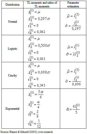
3. TL-Moments

3.1. TL-Moments of Probability Distributions

In this alternative robust modification of L-moments, the expected value E(X_r-j:r) is replaced by the expected value E(Xr+t₁−j:r+t₁+t₂). Thus, for each r we increase the sample size of random sample from the original r to r + t₁ + t₂ and we work only with the expected values of these r treated order statistics Xt₁+1_:r+t₁+t₂, Xt₁+2_:r+t₁+t₂, …, Xt₁+r_:r+t₁+t₂ by trimming the t₁ smallest and the t₂ largest from the conceptual sample. This modification is called the r-th trimmed L-moment (TL-moment) and is marked Thus, TL-moment of the r-th order of random variable X is defined

(30)

It is apparent from equations (30) and (1) that the TL-moments simplify to L-moments, when t₁ = t₂ = 0. Although we can also consider applications, where the values of trimming are not equal, i.e. t₁ ≠ t₂, we focus here only on symmetric case t₁ = t₂ = t. Then equation (30) can be rewritten

(31)

Thus, form example, is the expected value of median from conceptual random sample of sample size 1 + 2t. It is necessary here to note that is equal to zero for distributions, which are symmetrical around zero.

First four TL-moments have the form for t = 1

(32)

(33)

(34)

(35)

Note that the measures of location (level), variability, skewness and kurtosis of the probability distribution analogous to conventional L-moments (6)−(9) are based on

The expected value E(X_r:n) can be written using the formula (2). Using equation (2) we can re-express the right side of equation (31)

(36)

It is necessary to be noted here that is a normal the r-th L-moment without any trimming.

Expressions (32)-(35) for the first four TL-moments, where t = 1, can be written in an alternative manner

(37)

(38)

(39)

(40)

Distribution may be identified by its TL-moments, although some of its L-moments or conventional central moments do not exit; for example (the expected value of median of conceptual random sample of sample size three) exists for Cauchy’s distribution, although the first L-moment λ₁ does not exist.

TL-skewness and TL-kurtosis are defined analogously as L-skewness and L-kurtosis

(41)

(42)

3.2. Sample TL-Moments

Let x₁, x₂, …, x_n is a sample and is an ordered sample. Expression

(43)

is considered to be an unbiased estimation of the expected value of the (j + 1)-th order statistic X_j+1:j+l+1 in conceptual random sample of sample size (j + l + 1). Now we will assume that we replace the expression E(X_r+t−j:r+2t ) by its unbiased estimation in the definition of the r-th TL-moment in (31)

(44)

which we gain by assigning j → r + t − j − 1 a l → t + j in (43). Now we obtain the r-th sample TL-moment

(45)

i.e.

(46)

which is unbiased estimation of the r-th TL-moment Note that for each j = 0, 1, …, r − 1, values x_i:n in (46) are nonzero only for r + t – j ≤ i ≤ n – t −j due to the combinatorial numbers. Simple adjustment of the equation (46) provides an alternative linear form

(47)

For example, we obtain for r = 1 for the first sample TL-moment

(48)

where the weights are given by

(49)

The above results can be used to estimate TL-skewness and TL-kurtosis by simple ratios

(50)

(51)

We can choose t = nα representing the amount of the adjustment from each end of the sample, where α is a certain proportion, where 0 ≤ α < 0,5.

Table 3 contains the formulas for TL-moments and for the ratios of TL-moments and the formulas for parameter estimations obtained using the method of TL-moments of chosen probability distributions. More on the TL-moments is for example in [12].

Table 3. Formulas for TL-Moments and Ratios of TL-Moments and Formulas for Estimations of Parameters Taken by the Method of TL-Moments of Chosen Probability Distributions (t = 1)

4. Lognormal Curves

4.1. Three-Parametric Lognormal Curves

Random variable X has three-parametric lognormal distribution with parameters µ, σ² and θ, where –∞ < µ < ∞, σ² > 0, –∞ < θ < ∞, if its probability density function have the form

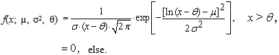(52)

Lognormal distribution with parameters µ, σ² and θ (beginning of distribution, theoretical minimum) is marked LN(µ, σ², θ). Probability density function of three-parametric lognormal distribution is asymmetric, positively skewed. Figures 1 and 2 show the graphs of the probability density function of three-parametric lognormal distribution depending on the values of the parameters of this distribution.

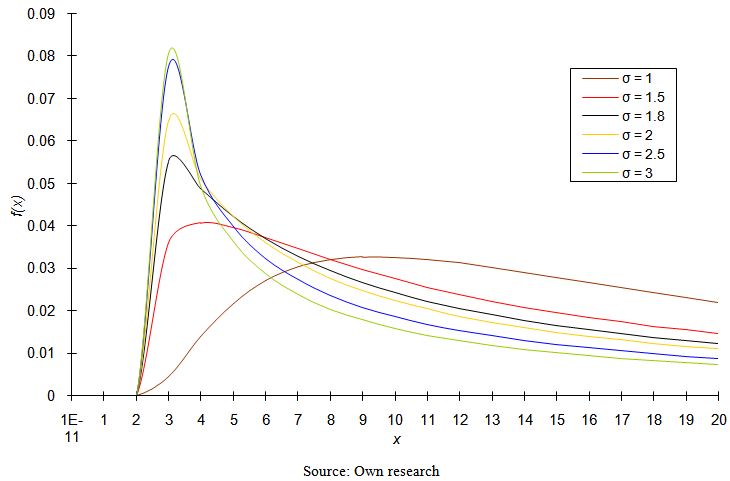
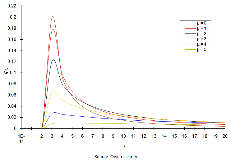Figure 1. Probability density function of three-parametric lognormal distribution for the values of parameters σ = 2 (σ2 = 4); θ = 2

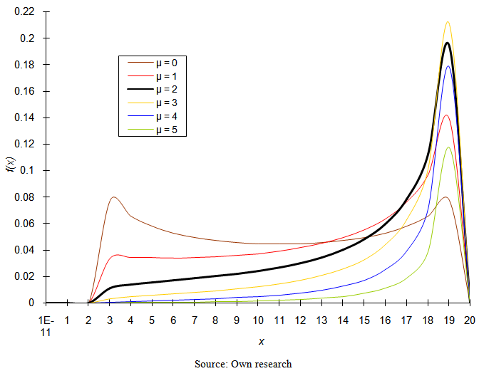
Figure 2. Probability density function of three-parametric lognormal distribution for the values of parameters μ = 3; θ = 2

Probability density function of three-parametric lognormal distribution is sometimes presented in the form

(53)

where it is valid between the expressions for probability density functions (52) and (53).

If we substitute θ = 0 (distribution minimum) into expressions for the probability density function of three-parametric lognormal distribution (52) and (53), we obtain formulas for the probability density function of two-parametric lognormal distribution.

Distribution function of three-parametric lognormal distribution has the form

(54)

If the random variable X has three-parametric lognormal distribution LN(µ, σ², θ), then the random variable

(55)

has normal distribution N(µ, σ²) and the random variable

(56)

has standardized normal distribution N(0; 1). Parameter μ is the expected value of random variable (55) and parameter σ² is the variance of this random variable. Parameter θ is the beginning of the distribution, i.e. theoretical minimum of the random variable X.

For the r-th common and central moments of three-parametric lognormal distribution have the form

(57)

(58)

specifically

(59)

(60)

We obtain the expressions for the expected value and variance of random variable X having three-parametric lognormal distribution from (57) and (58)

(61)

(62)

The expression for median

(63)

comes from the expression for 100 P% quantile of this distribution

(64)

Three-parametric lognormal distribution is unimodal with one mode

(65)

The relationship between the expected value, median and mode follows from the equations (61), (63) and (65)

(66)

which is typical just for positively skewed distribution.

The coefficient of variation of three-parametric lognormal distribution is a function of all three parameters µ, σ² and θ of this distribution

(67)

Gini’s coefficient of three-parametric lognormal distribution depends on all three parameters µ, σ² and θ of this distribution, too

(68)

Moment measurements of skewness and kurtosis depend on single parameter σ²

(69)

(70)

4.2. Four-Parametric Lognormal Curves

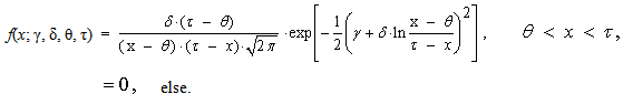
Random variable X has four-parametric lognormal distribution with parameters µ, σ², θ a τ, where –∞ < µ < ∞, σ² > 0, –∞ < θ < τ < ∞, if its probability density function has the form

(71)

Lognormal distribution with parameters µ, σ², θ a τ is marked LN(µ, σ², θ, τ). The probability density function of four-parametric lognormal distribution can have very different shapes depending on the values of the parameters of the distribution, see Figures 3–5. Distribution may be also bimodal for σ² > 2 and

Figure 3. Probability density function of four-parametric lognormal distribution for the values of parameters σ = 2 (σ2 = 4); θ = 2; τ = 20

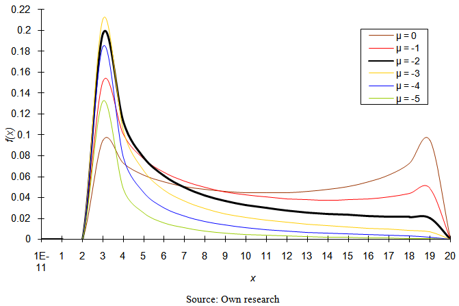Figure 4. Probability density function of four-parametric lognormal distribution for the values of parameters σ = 2 (σ2 = 4); θ = 2; τ = 20

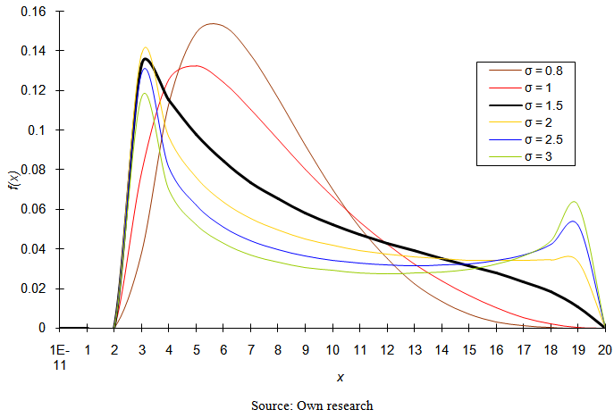Figure 5. Probability density function of four-parametric lognormal distribution for the values of parameters μ = –1; θ = 2; τ = 20

Probability density function of four-parametric lognormal distribution is often presented in the form

(72)

where it is valid between the expressions for probability density function (71) and (72)

If the random variable X has four-parametric lognormal distribution LN(µ, σ², θ, τ), then the random variable

(73)

has normal distribution N(µ, σ²) and the random variable

(74)

has standardized normal distribution N(0; 1). Parameter μ is therefore the expected value of a random variable (73) and the parameter σ² is the variance of this random variable. The parameter θ is the beginning of the distribution (theoretical minimum) of a random variable X and the parameter τ represents the end point of the distribution (theoretical maximum) of the random variable X.

More on the lognormal distribution is for example in [6], [7], [9] or [10].

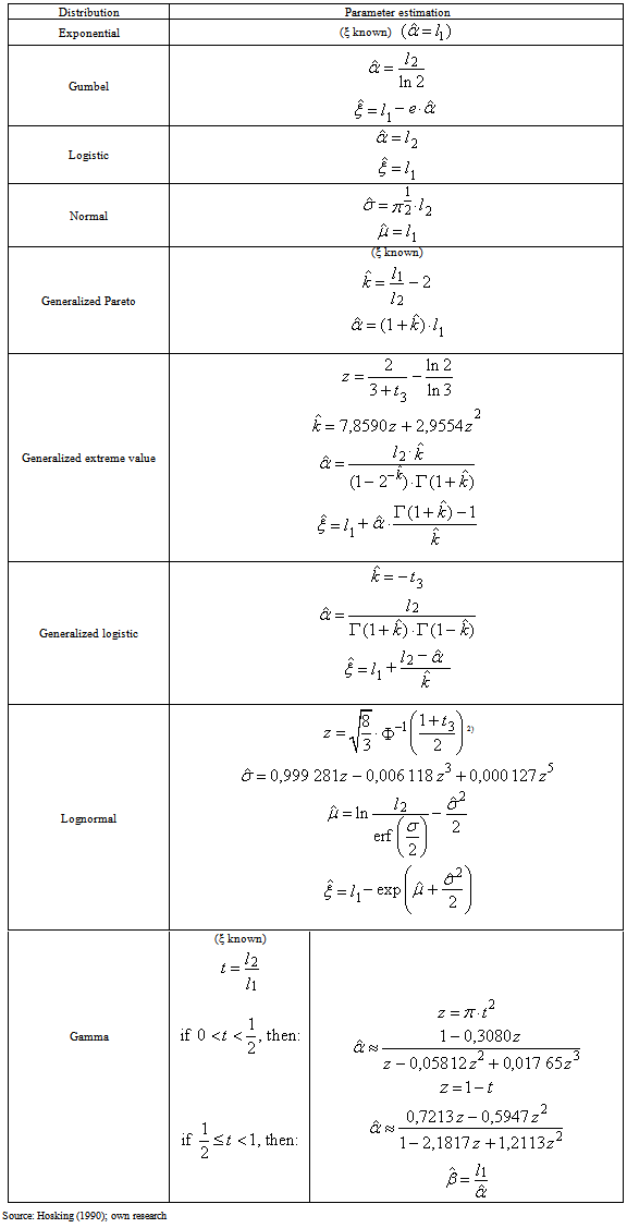
5. Methods of Parameter Estimation

We focus here only on the parameter estimation of three-parametric lognormal distribution, which is the basic theoretical probability distribution of this research. Various methods of parametric estimation can be used for estimating the parameters of three-parametric lognormal distribution. There are for example the maximum likelihood method, moment method, quantile method, Kemsley’s method, Cohen’s method, L-moment method, TL-moment method, graphical method, etc. We focus on maximum likelihood method and on lesser-known methods of parametric estimation, i.e. Kemsley’s method and Cohen’s method.

5.1. Maximum Likelihood Method

Let the random sample of the sample size n comes from three-parametric lognormal distribution with probability density function (52) or (53). Then the likelihood function has the form

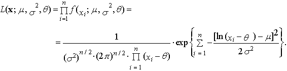(75)

We determine the logarithm of the likelihood function

(76)

We put in the equality to zero the first partial derivation of the logarithm of the likelihood function according to μ and according to σ² by

(77)

(78)

We obtain maximum likelihood estimations of the parameters μ and σ² for the given parameter θ after treatment

(79)

(80)

If the value of the parameter θ in known, we get the maximum likelihood estimations of the remaining two parameters of three-parametric lognormal distribution using the expressions (79) and (80). However, if the value of the parameter θ is unknown, the problem is more complicated. It can be proved that if the parameter θ closes to min{X_1, X_{2, …,} X_n}, then the maximum likelihood approaches to infinity. The maximum likelihood method is also often combined with Cohen’s method, where we put the smallest sample value to be equal to the 100• (n + 1)− ¹-percentage quantile

(81)

Equation (81) is then combined with a system of equations (79) and (80).

For solving of maximum likelihood equations (79) and (80) it is also possible to use satisfying the equation

(82)

where

(83)

where satisfy equations (79) and (80) with the parameter θ replaced by We may also obtain the limits of variances

(84)

(85)

(86)

Especially difficulties related with the use of the equations (79), (80) and (82) lead us to think about other methods.

5.2. Kemsley’s Method

Kemsley used the estimation method, which is a combination of moment and quantile methods of parametric estimation. This method of parametric estimation put into equality the sample quantiles and the corresponding theoretical quantiles of the probability distribution. We get the last equation so that we put sample average equal to the expected value of the probability distribution (“K” means Kemsley’s estimation).

(87)

(88)

(89)

Now we solve a similar system of equations as in the case of quantile method of parameter estimation and

(90)

The proposal for the solution of equation (90) determines approximately using Figure 6. Then we obtain the values of the remaining two parameters using the expressions

(91)

(92)

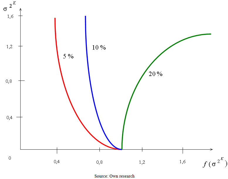Figure 6. Graph for Kemsley’s method of parametric estimation for p1 = 0,05; 0,10 and 0,20

5.3. Cohen’s Method of the Smallest Sample Value

It is known that parameter θ determines the beginning of three-parametric lognormal distribution. In this case, an appropriate estimation would be a function of the smallest sample value. This method constitutes an alternative to the method of maximum likelihood. This keeps the equations (79) and (80) and needed the third equation is based on the smallest sample value x_min. If the value x_min is contained n_min-times in the sample, then the sample quantile of order n_min/n in the third equation is putted into equality to the corresponding theoretical quantile of the distribution. Thus, Cohen’s method represents a combination of maximum likelihood method and the quantile method. We can get the parameter estimations obtained by Cohen’s method with the system of equations (“C” means Cohen’s estimation)

(93)

(94)

(95)

6. Appropriateness of the Model

It is also necessary to assess the suitability of constructed model or choose a model from several alternatives, which is made by some criterion, which can be a sum of absolute deviations of the observed and theoretical frequencies for all intervals

(96)

or known criterion χ²

(97)

where n_i are the observed frequencies in individual intervals, π_i are the theoretical probabilities of membership of statistical unit into the i-th interval, n is the total sample size of corresponding statistical file, n • π_i are the theoretical frequencies in individual intervals, I = 1, 2, ..., k, and k is the number of intervals.

The question of the appropriateness of the given curve for model of the distribution of wage is not entirely conventional mathematical-statistical problem in which we test the null hypothesis

H₀: The sample comes from the supposed theoretical distribution

against the alternative hypothesis

because in goodness of fit tests in the case of wage distribution we meet frequently with the fact that we work with large sample sizes and therefore the tests would almost always lead to the rejection of the null hypothesis. This results not only from the fact that with such large sample sizes the power of the test is so high at the chosen significance level that the test uncovers all the slightest deviations of the actual wage distribution and a model, but it also results from the principle of construction of the test. But practically we are not interested in such small deviations, so only gross agreement of the model with reality is sufficient and we so called “borrow” the model (curve). Test criterion χ² can be used in that direction only tentatively. When evaluating the suitability of the model we proceed to a large extent subjective and we rely on experience and logical analysis.

7. Database

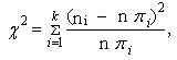
In the past L-moments were mainly used in hydrology, climatology and meteorology in the research of extreme precipitation, see for example [14]. There are mainly small data sets in this case. This study presents an application of L-moments and TL-moments on large sets of economic data, Table 4 presents the sample sizes of obtained sample sets of households.

Table 4. Sample Sizes of Income Distributions Broken Down by Relatively Homogenous Categories

The researched variable is the net annual household income per capita (in CZK) within the Czech Republic (nominal income). The data obtained come from a statistical survey Microcensus – years 1992, 1996, 2002, and statistical survey EU-SILC (The European Union Statistics on Income and Living Conditions) – the period 2004-2007, from the Czech Statistical Office. Total 168 income distributions were analyzed this way, both for all households of the Czech Republic together and also broken down by gender, country (Bohemia and Moravia, see Figure 7), social groups, municipality size, age and the highest educational attainment, while households are classified into different subsets according to the head of household, which is man in the vast majority of households. Sharply smaller sample sizes for women than for men in Table 4 correspond to this fact. Head of household is always a man in two-parent families of the type the husband and wife or two partners, regardless of the economic activity. In single-parent families of the type only one parent with children and in non-family households, where persons are not related by marriage or by union partner, nor parent-child relationship, the first decisive criterion for determining the head of household is the economic activity and the second aspect is the amount of money income of individual household members. This criterion also applies in the case of more complex types of households, such as the case of joint management of more than two-parent families.

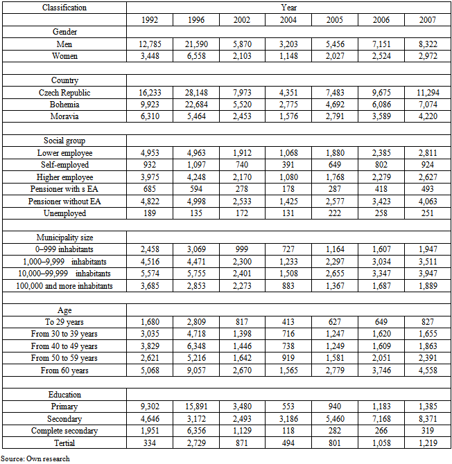
Figure 7. Map of the Czech republic (Bohemia and Moravia)

8. Results and Discussion

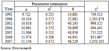
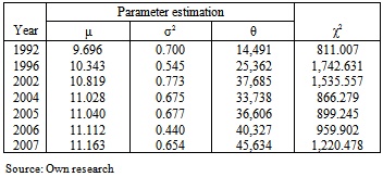
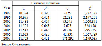
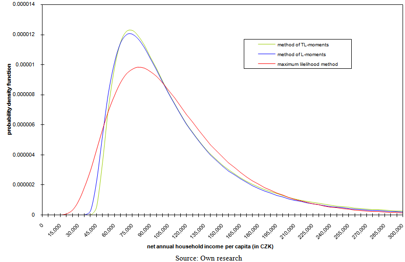
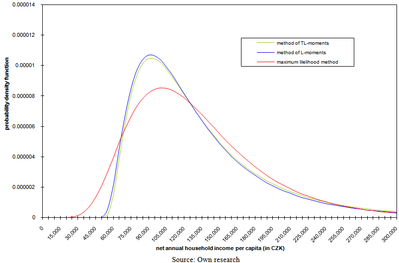
Method of TL-moments provided the most accurate results in almost all cases, with the negligible exceptions. Method of L-moments results as the second in more than half of the cases, although the differences between the method of L-moments and maximum likelihood method are not distinctive enough to turn in the number of cases where the method of L-moments came out better than maximum likelihood method.

Tables 5–7 are the typical representative of the results for all 168 income distributions. These tables provide the results for the total household set in the Czech Republic. They contain the estimated values of the parameters of three-parametric lognormal distribution, which were obtained simultaneously using the method of TL-moments, method of L-moments and maximum likelihood method, and the value of test criterion (97). This is evident from the values of the criterion that the method of L-moments brought more accurate results than maximum likelihood method in four of seven cases. The most accurate results were obtained using the method of TL-moments in all seven cases.

Table 5. Parameter Estimations of Three-Parametric Lognormal Curves Obtained Using the Method of TL-Moments of Point Parameter Estimation and the Value of χ2 Criterion

Table 6. Parameter Estimations of Three-Parametric Lognormal Curves Obtained Using the Method of L-Moments of Point Parameter Estimation and the Value of χ2 Criterion

Table 7. Parameter Estimations of Three-Parametric Lognormal Curves Obtained Using the Maximum Likelihood Method of Point Parameter Estimation and the Value of χ2 Criterion

The estimation of the value of the parameter θ (beginning of the distribution, theoretical minimum) obtained using the maximum likelihood method is negative in 1992 and 2005–2007. This means that three-parametric lognormal curve gets into negative values initially its course in terms of income. Since at first the curve has very tight contact with the horizontal axis, it does not matter good agreement of model with real distribution.

Figures 8–10 allow the comparison of these methods in terms of model probability density functions in choosing years (1992, 2004 and 2007) for the total set of households throughout the Czech Republic together. It should be noted at this point that other scale is on the vertical axis in Figure 8 than in Figures 9 and 10 for better legibility, because income distribution just after the transformation of the Czech economy from a centrally planned to a marked economy still showed different behaviour (lower level and variability, higher skewness and kurtosis) than the income distribution closer to the present. It is clear from these three figures that the methods of TL-moments and L-moments bring the very similar results, while the probability density function with the parameters estimated by maximum likelihood method is very different from model probability density functions constructed using the method of TL-moments and the method of L-moments.

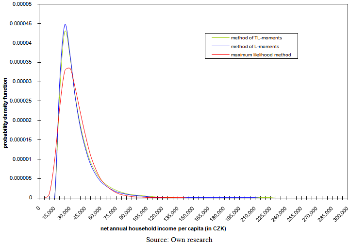Figure 8. Model probability density functions of three-parametric lognormal curves in 1992 with parameters estimated using three various robust methods of point parameter estimation

Figure 9. Model probability density functions of three-parametric lognormal curves in 2004 with parameters estimated using three various robust methods of point parameter estimation

Figure 10. Model probability density functions of three-parametric lognormal curves in 2007 with parameters estimated using three various robust methods of point parameter estimation

Figure 11 also provides some comparison of the accuracy of these three methods of point parameter estimation. It represents the development of the sample median and the theoretical medians of lognormal distribution with parameters estimated using the method of TL-moments, method of L-moments and maximum likelihood method in the researched period again for the total set of households of the Czech Republic. It is also clear from this figure that the curve representing the course of the theoretical medians of lognormal distribution with parameters estimated by methods of TL-moments and L-moments are more tightly to the curve showing the course of sample median compared with the curve representing the development of theoretical median of lognormal distribution with parameters estimated by maximum likelihood method.

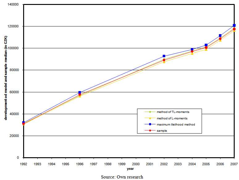Figure 11. Development of model and sample median of net annual household income per capita (in CZK)

Figures 12–14 show the development of the model probability density functions of three-parametric lognormal distribution again with parameters estimated using three researched methods of parameter estimation in the analysed period for total set of households of the Czech Republic. Also, in view of these figures income distribution in 1992 shows a strong difference from the income distributions in next years. Also here, we can observe a certain similarity of the results taken using the methods of TL-moments and L-moments and considerable divergence of the results obtained using these two methods of point parameter estimation from the results obtained using the maximum likelihood method.

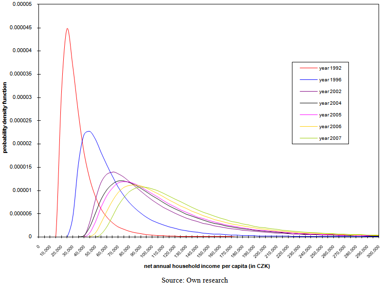
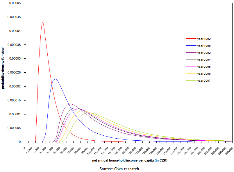Figure 12. Development of probability density function of three-parameter lognormal curves with parameters estimated using the method of TL-moments

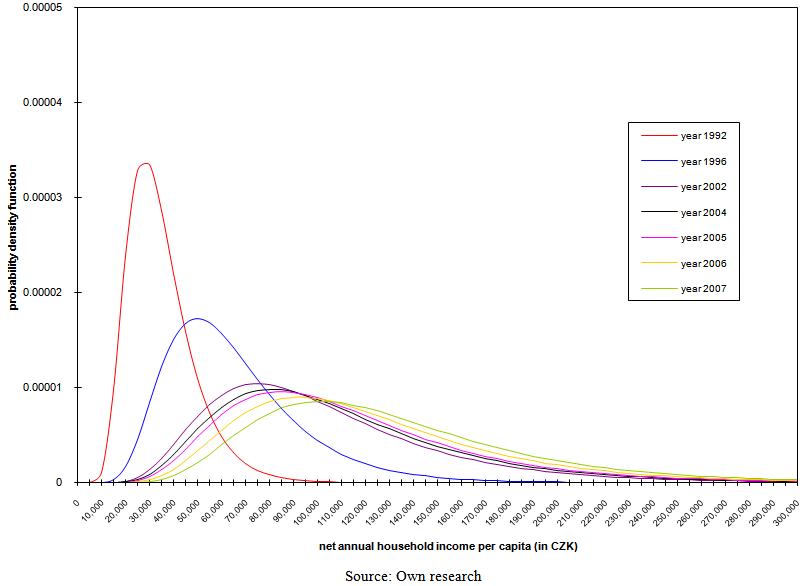
Figure 13. Development of probability density function of three-parameter lognormal curves with parameters estimated using the method of L-moments

Figure 14. Development of probability density function of three-parameter lognormal curves with parameters estimated using the maximum likelihood method

Figures 15-17 then represent the model relative frequencies (in %) of employees by the band of net annual household income per capita in 2007 obtained using three-parametric lognormal curves with parameters estimated by the method of TL-moments, method of L-moments and maximum likelihood method. These figures also allow some comparison of the accuracy of the researched methods of point parameter estimation compared with Figure 18, where are the really observed relative frequencies in individual income intervals obtained from a sample.

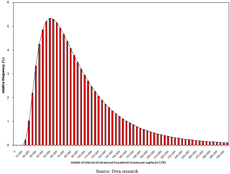Figure 15. Model ratios of employees by the band of net annual household income per capita with parameters of three-parametric lognormal curves estimated by the method of TL-moments in 2007

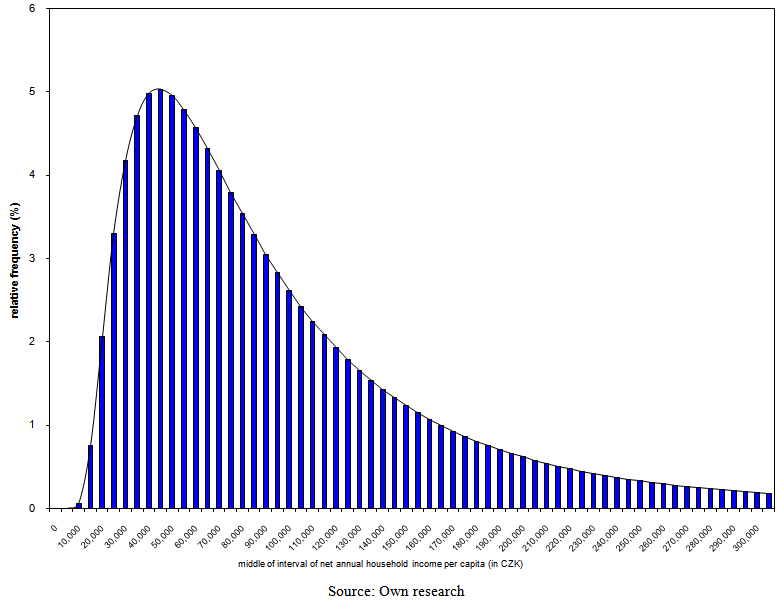Figure 16. Model ratios of employees by the band of net annual household income per capita with parameters of three-parametric lognormal curves estimated by the method of L-moments in 2007

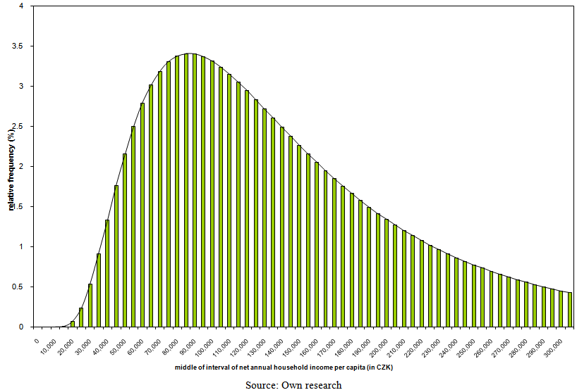Figure 17. Model ratios of employees by the band of net annual household income per capita with parameters of three-parametric lognormal curves estimated by the maximum likelihood method in 2007

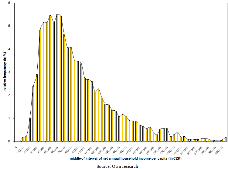Figure 18. Sample ratios of employees by the band of net annual household income per capita in 2007

9. Conclusions

Relatively new class of moment characteristics of probability distributions were here introduced. There are the characteristics of location (level), variability, skewness and kurtosis of probability distributions constructed using L-moments and TL-moments that are robust extension of L-moments. Own L-moments have been introduced as a robust alternative to classical moments of probability distributions. However, L-moments and their estimations lack some robust features that belong to TL-moments.

Sample TL-moments are linear combinations of the sample order statistics, which assign zero weight to a predetermined number of sample outliers. Sample TL-moments are unbiased estimations of the corresponding TL-moments of probability distributions. Some theoretical and practical aspects of TL-moments are still the subject of research or they remain for future research. Efficiency of TL-statistics depends on the choice of α, for example, have the smallest variance (the highest efficiency) among other estimations for random samples from normal, logistic and double exponential distribution.

The above methods can be also used for modeling the wage distribution or other analysis of economic data (among other methods, see for example [15] or [16]).

ACKNOWLEDGEMENTS

This paper was subsidized by the funds of institutional support of a long-term conceptual advancement of science and research number IP400040 at the Faculty of Informatics and Statistics, University of Economics, Prague, Czech Republic.

Notes

1) I_x(p, q) is incomplete beta function

2) Φ⁻¹(·) is quantile function of standardized normal distribution