-
Paper Information
- Next Paper
- Paper Submission
-
Journal Information
- About This Journal
- Editorial Board
- Current Issue
- Archive
- Author Guidelines
- Contact Us
American Journal of Mathematics and Statistics
p-ISSN: 2162-948X e-ISSN: 2162-8475
2014; 4(2): 51-57
doi:10.5923/j.ajms.20140402.01
Analysis of Compositional Time Series from Repeated Surveys
 Abstract
 Reference
 Full-Text PDF
 Full-text HTML
Etebong P. Clement
Department of Mathematics and Statistics University of Uyo, P.M.B.1017 Uyo, Uyo, Nigeria
Correspondence to: Etebong P. Clement, Department of Mathematics and Statistics University of Uyo, P.M.B.1017 Uyo, Uyo, Nigeria.
| Email: |  |
Copyright © 2012 Scientific & Academic Publishing. All Rights Reserved.
A compositional time series is a multivariate time series in which each of the series has values bounded between zero and one and the sum of the series equals one at each time point. Data with such characteristics are observed in repeated surveys when a survey variable has a multinomial response but interest lies in the proportion of units classified in each of its categories. The main approach to analyzing Compositional Time Series data has been based on the application of an initial transform to break the unit sum constraint. Box-Cox transformation originally was envisioned as a panacea for simultaneously correcting normality, linearity and homoscedasticity. However, one thing is clear; that seldom does this transformation fulfill the basic assumptions as originally suggested. This paper aims at reviewing works relating to these transformations with some modifications and illustrative example as would be applicable to the analysis of compositional time series data.
Keywords: Box-Cox transformation,Compositional time series,Multinomial response, Repeated surveys
Cite this paper: Etebong P. Clement, Analysis of Compositional Time Series from Repeated Surveys, American Journal of Mathematics and Statistics, Vol. 4 No. 2, 2014, pp. 51-57. doi: 10.5923/j.ajms.20140402.01.
Article Outline
1. Introduction
- Repeated surveys produce time series
 comprising estimates of the unknown target series
  . If a survey is repeated at times
  then multinomial responses at each time
  , lead to compositions. A composition is a vector of non-negative components summing to a constant, usually a unity. Symbolically, a vector
  such that:
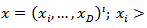
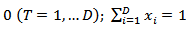 is a composition. A time series of composition is referred to as a compositional time series (CTS).A compositional time series (CTS) is defined as a multivariate time series in which each of the series has values bounded between zero and one and the sum of the series equals one at each time point. Data with such characteristics are observed in repeated surveys when a survey variable has a multinomial response but interest lies in the proportion of unit classified in each of its categories. Therefore, the survey estimates are proportions of a whole subject to a unity-sum constraint. A repeated survey is a sample survey which is performed more than once with essentially the same questionnaire or schedule but not necessarily with the same sample units. Many repeated surveys are based on a rotating panel design in which K panels of sampling units are investigated at each survey round (time point) and panels are replaced in a systematic manner, according to the rotating pattern of the survey design. In these surveys, elementary design unbiased estimates
  , for the population parameters
  , can be obtained from each rotation group. A rotation group is a set of sampling units that joins and leaves the sample at the same time [1].A repeated survey enables estimation of changes for the population as well as cross-sectional estimate. Monitoring and detecting important changes will usually be a key reason for sampling in time. Common frequencies for repeated survey are monthly, quarterly and annual. However more frequent sampling may be adopted as in the opinion polls leading up to an election and monitoring Television or Radio rating [2]. Some examples of repeated surveys are monthly labour force surveys in Australia. Quarterly surveys include the labour force survey in U.K and Ireland and many business surveys. Annual surveys include the Annual Survey of Manufacturers of the U.S. Census Bureau enumerates a fixed panel of economic establishments for five survey years. Establishments are selected with probabilities proportionate to size using Poisson sampling. The June Enumerative Survey of the National Agricultural Statistics Service is a yearly survey of agricultural activities. The farm costs and returns survey, also of the National Agricultural Statistics Service, enumerates a stratified simple random sample of farms each year. In a repeated survey there is not necessarily any overlap of the sample for different occasions. A rotating panel surveys also uses a sample that is followed over time, but the focus is on estimates at aggregate levels. When the emphasis is on estimates for the population an independent sample may be used on each occasion, which is often the case when the interval between the surveys is quite large. An option is to use the same sample at each occasion, with additions so that the sample estimates refer to the current population. For monthly or quarterly surveys the sample is often designed with considerable overlap between successive surveys. The sample overlap will reduce the sampling variance of estimates of change and reduce costs. Many important surveys are conducted repeatedly to give estimates of the level or mean for several time periods. Repeated surveys can provide estimates for each time periods
  . A major value of repeated surveys is in their ability to provide estimates of change. The simplest analysis of change is the estimate of one period change
  . In a monthly survey this corresponds to one month change. For a survey conducted annually this corresponds to annual change. In general, therefore the change
  time periods apart can be estimated as the difference at
  .The focus is often on
  , but for a survey repeated on a monthly basis changes for
  are also commonly examined [2]. Having sample overlap at
  will usually lead to a positive correlation between the estimates. Since
 having sample overlap reduces the variance of
  compared with having no sample overlap. [3] considered the components of change in a repeated survey [4-6] give a general review of issues in the design and analysis of repeated surveys. [7] cover many of the important issues associated with panel surveys. [8-10] review estimation issues for repeated surveys. The focus of this paper is on compositional data from repeated surveys. Data of this kind frequently arise in disciplines as disparate as biology, demography, ecology, economics, geology and politics. Examples are: the percentage of different species of fish recorded in a lake at different instants in time, the composition of monthly immigration to a city according to the country of origin, the daily market share at the end of trading, the breakdown of household monthly consumption by type of item in budget surveys and the results of opinion polls conducted at different times during an election campaign [11]. In this paper we give a detailed review of developments in the field of the statistical analysis of compositional time series (CTS). Historically, the main approach to analyzing CTS data has been based on the application of an initial transform to break the unit sum constraint, followed by the use of standard time series techniques. The inverse transformation is then used on the derived results to obtain results pertinent to the original sample space. That is, the inverse transformation is applied to obtain the equivalent inferential results for the original compositional time series (CTS).This approach was first discussed by [12] in the context of analyzing CTS from repeated sample surveys. In [12-14], the authors first proved that such an approach is in variant to the choice of the component used as the common divisor in the additive log ratio (alr) transformation. Secondly, assuming normality for the distribution of
  , they obtained forecasts for the original CTS
  by calculating the mean of the corresponding additive logistic distribution numerically. In this paper two methods of analyzing CTS is discussed: The direct modeling in the simplex, and transformation of the simplex. An attempt is made at reviewing the works relating to the transformation of the simplex with some modifications.
 2. Compositional Time Series
- Let
 | (1) |
 , and assume that observations are taken at equally spaced time intervals
  .Let
.Let | (2) |
 based on data collected at time
  .Repeated surveys produce time series
  comprising estimates of the unknown target series
  . According to [1] focusing on the unknown population vector
  , it is natural to imagine that knowledge of
  conveys useful information about
  but without implying that it is perfectly predictable from
  .One way of representing this situation is by considering
  being a random variable which evolves stochastically in time following a certain time series model, as was first proposed for univariate survey analysis by [15-17]The survey estimates
  of (1) and (2) can then be expressed as
  | (3) |
 ,
,  and
and  are random processes and
  are the sampling errors such that
  and
and  .Many variables investigated by statistical agencies have a multinomial response and interest lies in the estimation of the proportion of units classified in each of the categories. If this is the case, the vector of proportion sums to one and forms what is known as a composition. A composition is a vector of non-negative components summing to a constant, usually 1, or put symbolically, a vector
  such that
  .A time series of compositions is referred to as a Compositional Time Series (CTS). A Compositional Time Series is a sequence of vectors
 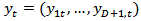 each belonging to the simplex
  .If a survey is repeated at time
  , then multinomial response at each time at
  say constitute compositions.
 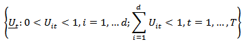 which forms a multivariate time series. The transformation of the series produces a multivariate time series defined on
  at each time point
  which can be analysed using standard methods. In particular [13] examined the use of ARMA models on the transformed series defined by
 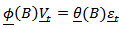 .
. In the multivariate case, the ideas of [18] who give a very simple procedure for choosing, estimating and testing such models is always followed. However, it is always necessary to consider if the choice of reference variable in any way influences the analysis. Consequently, [12] proves the following results. (i) Let
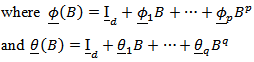
 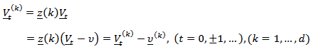 where
where  is given by
 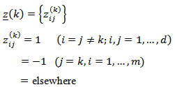 and
and  , then if
  follows a multivariate ARMA
  process of dimension
  then
then  is also multivariate ARMA
  . The roots of the determinantal equations of both the AR and MA components from the two models are identical so that the stationarity and invertibility conditions remain consistent. (ii) Consider the compositional time series
  where
where 
 follows an ARMA (p, q) process. Then each ARMA model
  represents the same model for
  , except that the elements of
  and associated parameters have been permuted. That is, the model for
  is totally invariant to the choice of reference variable. The consequences of results (i) and (ii) is that any component of
  may be selected as the reference variable without affecting the final results. In what follows, we assume that the reference variable is
  . The application of compositional data to modelling and forecasting is straight forward when the argument of [19] is followed. Let the series
  be transformed to
  .
.
 is then modeled by the vector ARMA
  , forecasts for
  can be obtained. Let the
  -step a head forecast
  of
of  be denoted by
  and its covariance matrix
  , a “naïve” forecast for
  as:
as: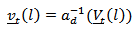 Assuming normality for the distribution of
  so that
 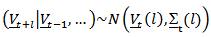 . The optimum forecast of
  may be obtained numerically by calculating the mean of
  or
or  may be approximated. Also a confidence region for
  may be obtained following standard multivariate theory, though the confidence region will not centered at
  .A 100
  confidence region for
  according to [13] can be formed from
 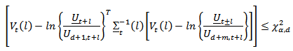 where
where  is the
  point of a
  distribution, by mapping points from
  onto the simplex
  .Also forecasts for either the ratios
  or generally the log-ratios may be obtained.
  where
where 
3. Analyzing Compositional Time Series
- Two methods of analyzing compositional time series will be explored, namely: Direct method and transformation method. Under the transformation methods of analysis, we shall examine two techniques: Box and Cox transformation and the log-ratio transformation. Again, the log ratio transformation shall be viewed under: (i) additive log ratio (alr) transformation (ii) centered log ratio transformation (clr) and (iii) isometric log ratio transformation.
3.1. Direct Modeling in the Simplex
- Around the same time as the publication of [12] and [20-21] introduced a different approach to analyzing CTS, which had also been inspired by some of the earlier ideas of Aitchison. There and in [22], the authors developed space state models which could be used to model CTS data directly in the simplex. The distribution of the CTS conditioned on the unobserved state was assumed to be Dirichlet. The state distribution was assumed to be Dirichlet conjugate. This was a new generalization of the Dirichlet distribution proposed by them in order to allow for dependence between the components. A vector of continuous proportions consists of the proportions of some total accounted for by its constituent components (compositions). We consider the situations where time series data are available and where interest focuses on the proportions rather than the actual amounts. A state space model for time series of compositions conditionally on the unobserved state, the observation are assumed to follow the Dirichlet distribution, often considered to be the most natural distribution on the simplex. The state follows the Dirichlet conjugate distribution.Let
 be a vector of continuous proportions, namely a vector with positive components such that
  .Where
  is a
is a  - vector of 1s.Then
  follows the Dirichlet distribution if it has the density
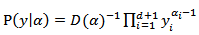 | (4) |
 where
where  for
for  and
and 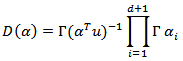 is the Dirichlet function, a
  - dimensional analogue of the beta function. We denote this situation by
  .The sample space is the d-dimensional simplex
  ;
;  Expressing (4) in exponential family form, we have: Let
 and
and  Z is the vector of symmetric log ratios (clr) and Z = clr (y)Also let
  where
where  so that
  . Then density (4) becomes:
  | (5) |
 and the parameters space is
 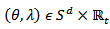 . The purpose of this reparameterization according to [22] is to separate the effects of location
  and spread
  as far as possible.
 3.2. Transformation Method
- The sample space of a composition
 is referred to as the simplex
  . It has been known since the days of [23] that normal statistical methods are not applicable to element of the simplex (the compositions).The major way, following the ideas of Aitchison of resolving these problems has been through transformation.
 3.2.1. Box-Cox Transformation
- [24] introduced the use of the well-known Box-Cox transformation as an alternative to the additive log ratio (alr) transformation. The Box-Cox transformation has the advantage of including the alr transformation as a special case. However, the only application of this approach known is that presented in [25]. These authors modeled the Box-Cox transformed data using dynamic linear models incorporating a rich class of distributions for the errors based on scale mixtures of multivariate normal distributions. This general class of distributions includes as special cases the multivariate normal, student-t, logistic and stable distributions, among others. [25] used the same complex procedure as those proposed in [26] to carry out model selection and inference. They illustrated their approach using two CTS; the mortality data from Los Angeles (analyzed previously by [26] and a CTS on vehicle production which had been previously analyzed by [21].[27] introduced a family of power transformation such that the transformed values are a monotonic function of the observations over some admissible range and indexed by
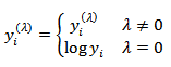 | (6) |
 . However, this family has been modified by [28] to take account of the discontinuity at
  , such that
 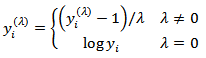 | (7) |

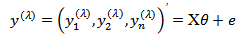 where
where  is a matrix of known constants,
  is a vector of unknown parameters associated with the transformed values and
 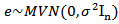 is a vector of random errors. The transformation in equation (7) is valid only for
  and, therefore, modifications have had to be made for negative observations. [28] proposed the shifted power transformation with the form
 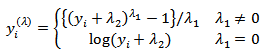 | (8) |
 is the transformation parameter and
  is chosen such that
  .[29] introduced the so-called modulus transformation which is considered to normalize distributions already possessing some measure of approximate symmetry and carries the form
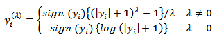 | (9) |
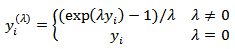 | (10) |
 with unbounded support such as the normal distribution can be included. For
  , the extension is:
 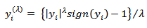 | (11) |
 in equations (6) – (9) is restricted according to whether
  is positive or negative. This implies that the transformed values do not cover the entire range
  and, hence, their distributions are of bounded support. Consequently, only approximate normality is to be expected.It is also remarked that since [28] transformation, other modifications of the transformation for special applications and circumstances had been made, but for most researchers, the original Box-Cox transformation of equation (7) suffices and is preferable due to computational simplicity.
 3.2.2. Log Ratio Transformation
- Let
 denote the family of all real D x D matrices such that
 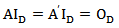 Let
Let  and
and  . We defined the product
  as:
as: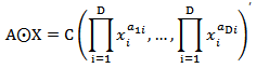 The function
  is an endomorphism of the vector space
  . Moreover, any endomorphism of
  can be written in this form. The matrix associated to identity endomorphism is the well-known centering matrix
 of order
  . (i) Additive Log ratio Transformation (alr)The alr transformation of index
 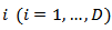 denoted by alr(x) is the one-to-one transformation from
  to
to  define as:
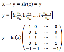 where
where  and
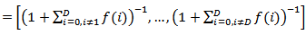
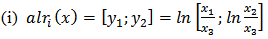
and  The inverse denoted
  or (gal) is defined as:
  where gal means generalized additive logistic transformation
 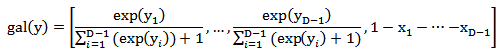 The additive log ratio transformation is asymmetric in the parts of the compositions. (ii) Centered Log Ratio Transformation (clr)The centered (or symmetric) log ratio transformation denoted by clr is the function from the compositional space
  to
to  , defined by:
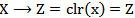
 where
where  and
and  is the geometric mean
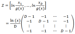
  of x. The inverse denoted by
  is defined by
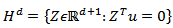
  This transformation is symmetric in the parts of the composition. The transformation maps
  in the subspace
 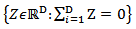 of
of  , which can be seen to be a hyperplane through the origin of
  , orthogonal to
  (vector of units). This subspace has dimension
  . If
. If  be any orthonormal basis of
  and if
  be the
  matrix
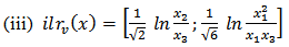
  .(iii) Isometric Log Ratio Transformation (ilr)The isometric log ratio transformation denoted by
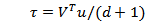
 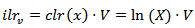 .For a given matrix V of D rows and (D-1) columns such that
  (identity matrix of
  elements) and
 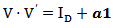 where
where  may be any value and 1 is a matrix full of ones. Alternatively,
 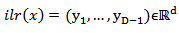 where d=D-1where
 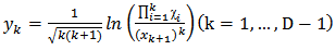 The inverse denoted by (ilr)-1 is defined as:
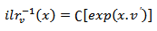
 ,where
 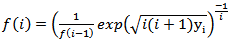 and
and  Let evaluation the log ratio transformations when D=3 and 4. For
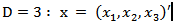
 where
where 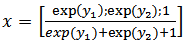
 where
where 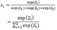
 where
where 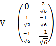 Again if D=4, that is,
  then the resulting vectors of the different transformations are the following:
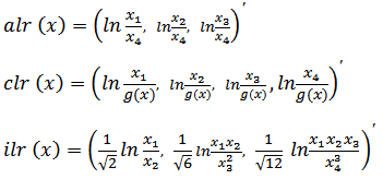 where g(x) is the geometric mean as defined earlier. It is very important to emphasize that all these transformations -
 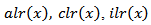 and its inverses are one-to-one linear transformations between the compositional vector space
  and the real vector space
 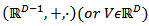 with the natural structure. Vectors
 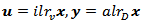 and
and  associated with the same composition
  are related by the following linear relationship expressed in matrix form.1.
  2.
2.  3.
3.  and
and  where
where  is the
  matrix
  , with
 .
.4. Conclusions
- The Box-Cox transformation has been widely used since it was first proposed. It has inspired a large amount of research on its applicability as well as on the drawbacks arising from its usage. However, one thing is clear; that seldom does this transformation fulfill the basic assumptions of linearity, normality and homoscedasticity simultaneously as originally suggested by [28]. A review of alternatives approaches is presented with modifications and illustrations useful to the analysis of compositional time series data.