Viviane Y. Naimy
Professor of Finance, Faculty of Business Administration and Economics, Notre Dame University, Louaize, Lebanon
Correspondence to: Viviane Y. Naimy, Professor of Finance, Faculty of Business Administration and Economics, Notre Dame University, Louaize, Lebanon.
| Email: |  |
Copyright © 2012 Scientific & Academic Publishing. All Rights Reserved.
Abstract
This paper presents a detailed analysis of Paris Stock Market’s volatility using GARCH(1,1) model after the 2007 financial crisis. A long term volatility rate of 1.696% per day has been calculated using the maximum likelihood methods to estimate the GARCH(1,1) parameters. This rate is compared to 1.39% before the crisis (for the period 2001-mid 2007). The model appeared strong and robust by removing autocorrelation from returns. Variance targeting procedures was used to confirm the values of GARCH(1,1) parameters. The EWMA model was also implemented and compared to the GARCH(1,1) model, where the objective functions in both models turned out to be close.
Keywords:
GARCH(1,1), EWMA, Variance Targeting, Paris Bourse, Maximum Likelihood Methods
Cite this paper: Viviane Y. Naimy, Parameterization of GARCH(1,1) for Paris Stock Market, American Journal of Mathematics and Statistics, Vol. 3 No. 6, 2013, pp. 357-361. doi: 10.5923/j.ajms.20130306.09.
1. Introduction
Risk managers cannot assume that asset prices move with a constant volatility. For a better forecasting, it is important to monitor volatility and keep tracking of variations through time. Among the most efficient models dealing with the conditional variance we name the ARCH (Autoregressive Conditional Heteroskedasticity) model of Engle (1982) then the GARCH (Generalized Autoregressive Conditional Heteroscedasticity) framework initiated by Bollerslev (1986). The ARCH allows the conditional variance to change over time as a function of past errors. Only the unconditional variance is left constant. Models using an estimate of the conditional variance as a proxy for the risk premium were developed by Engle, Lilien and Robins (1985). Therefore the comparison of volatility models became difficult because modeling heteroscedasticity is not an easy task. Only models with strong forecasting abilities have been used. Some models, in an in-sample analysis, illustrated the asymmetrical reaction of volatility to both positive and negative changes in returns but were not enough significant (Hansen R. and A. Lunde (2001)). There are different volatility models however and as tested by Hansen R. and A. Lunde (2001), they did not point to a single best model among the 330 they have assessed and they concluded that the best models did not provide a significantly better volatility forecast than the GARCH(1,1) model.The purpose of this paper is to study the volatility of Paris Stock Market (Bourse de Paris or Paris Bourse) through estimating GARCH(1,1) parameters. Such work was never performed after the 2007 financial crisis. Irrespective of whether Paris Stock Market is enough liquid, efficient or strongly capitalized, this market deserves a systematic analysis that can help investors and risk managers to assess its volatility. Therefore, we will describe and model the needed procedures to parameterize GARCH(1,1) for Paris Stock Market. This type of model is useful in modeling several different economic phenomena. In Engle (1982), Engle (1983) and Engle and Kraft (1983), models for the inflation rate were constructed[1]. The same principal was applied to the foreign exchange market. This paper serves as a guide for GARCH(1,1) approach using maximum likelihood methods and variance targeting procedure (Engle R. and Mezrich J. (1996)). These methods involve algorithm practice to determine the parameter values that maximize the chance that the historical data will occur. The paper proceeds as follows. In section 2 a panoramic and simplified review of ARCH and GARCH(1,1) is presented. The sample selection together with the model implementation using the maximum likelihood estimation of GARCH parameters are methodically evaluated and analyzed in section 3. Some test results are depicted in section 4 in order to check the GARCH(1,1) efficiency in the conditional variance equation for Paris Stock Market. An implementation of the variance targeting is also parameterized in this section. The paper then concludes the empirical findings.
2. A Simplified Panoramic Review of ARCH(m), EWMA, GARCH(1,1) and other Models
The Arch (m) model was first suggested by Engle (1982) where the estimate of the variance is based on a long-run average variance and m observations. The older the observation the less weight it is given. The simplification of the variance rate  formula at the end of day n-1 is given by equation (1) below:
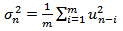 | (1) |
Where ui is defined as the percentage change in the market variable between the end of day i-1 and the end of day i. In this case  is assumed to be zero[2]. This gives equal weight to all the percentage changes in the market variable. Equation (2) allocates different weights to these changes:
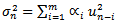 | (2) |
 and
and 
 represents the weight given to the change i days ago. More weight is given to recent data therefore
  when i > j. Assuming the presence of a weighted long-term average variance rate, equation (2) takes the form
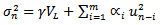 | (3) |
where Putting
  , ARCH (m) model can be written
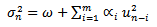 | (4) |
If the weights decrease exponentially as we move back through time, the exponentially weighted moving average, EWMA, which is a particular case of ARCH(m), is then used. The advantage of the EWMA approach is that few data are needed: the current estimate of the variance,  , and the most recent observation on the value of the market variable,
  .In this specific case:
  where 0 < λ < 1. Such weighting structure implies an updated volatility equal to
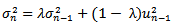 | (5) |
Equation (5) can also be written[3]  | (6) |
For large m, the term  can be ignored since it becomes close to zero. Therefore equation (6) is similar to equation (2)[4]. Each weight is λ times the previous one and they decline at a rate λ as we go back in time. The EWMA is an efficient approach to track changes in the volatility. A λ of 0.94 is generally used[5] for updating daily volatility estimates.The general GARCH(p,q) model calculates
  from the most recent p observations on u2 and the most recent q estimates of the variance rate. The (1,1) in GARCH(1,1) indicates that
  is based on the most recent observation of u2 and the most recent estimate of the variance rate. The calculation of
  in GARCH(1,1) equation is based on a long run average variance rate, VL, on
  and
and  :
: | (7) |
Where  For a stable GARCH(1,1) process, we need
  in order for
  to be positive. When
  and
and  and GARCH(1,1) reduces to EWMA. In cases where
  is negative, the GARCH(1,1) is not stable so it is recommended to switch to the EWMA model. Equation (7) can be written
 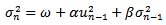 | (8) |
This is the equation on which we will be working to estimate  of Paris Bourse.It is important to mention the presence of other useful volatility models although the GARCH(1,1) model was never outperformed (Hansen R. and A. Lunde (2001)). We list the alternative GARCH-type models with the conditional mean: zero mean, non-zero constant mean and GARCH - in-mean (σ2) together with the alternative GARCH-type models with the conditional variance: ARCH, GARCH, IGARCH, Taylor/Schwert, A-GARCH, NA-GARCH, V - GARCH, GJR-GARCH, log-GARCH, EGARCH, NGARCHa, A-PARCH, GQ-ARCH, H-GARCH, and Aug - GARCHb.
3. Data and Sample Selection
The Paris Bourse has been computerized in 1990 with continuous trading through the CAC (Cotation Assistée en Continu) system. The opening price is determined by a preopening mechanism with an initial auction where market makers and floor traders have no special obligations. We will be estimating the volatility using the CAC 40 indicator which is the most commonly used index for Paris stock exchange market. This index includes the price of the 40 largest companies listed in France. It is based on a free-float market capitalization with a base value of 1,000 that started on December 31, 1987.The data were extracted from Bloomberg. A total of 1,515 daily observations of CAC 40 (closing value) were collected between September 3, 2007 and August 1, 2013. The purpose being the parameterization of GARCH(1,1) model after the 2007 financial crisis for Paris stock market.
3.1. Methodology
We will use the maximum likelihood method for the calculation. This involves the selection of the parameters that maximize the likelihood of the data occurring. We define the estimate of the variance for day  . Assuming that the conditional probability distribution of ui on the variance is normal, then the likelihood of ui to be observed is the probability density function for the variable X = ui for m observations is
 | (9) |
The likelihood of m observations occurring in the order they are observed is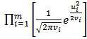 | (10) |
Taking logarithms of the expression in equation (10) and ignoring the constant multiplicative factors, equation (10) can be written as follow: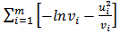 | (11) |
Therefore the value that maximizes this expression is the best estimate of v. We will use an algorithm procedure to find the parameters that maximizes the above equation.
3.2. Implementation
The GARCH(1,1) spreadsheet is based on trial estimates of  . The calculation of ui is based on the relative change of the CAC value[6]. As for the variance estimate we started at day 3 by setting the variance v3=σ22. From day 4 to day 1,515 we implemented equation (8). Equation (11) was then used in a separate column based on the variance estimates previously calculated[7]. In fact we are interested in choosing
  that maximizes equation (11). This involves an algorithm procedure. We used Solver where the changing cells were
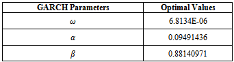
  and the objective cell contains equation (11) to be maximized.These values turn out after 1,000 iterations to be:The maximum value[8] of equation (11) is
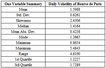
 The long term volatility[9], deduced from equation (7), is 1.696% per day. The below graph illustrates the GARCH(1,1) volatility variations over the last six years for Paris Bourse. The fifth percentile was above 1% per day and the median reached 1.416% while the highest registered rate exceeded 5.4% per day. Table 2 summarizes the volatility rates statistics for the last six years.
Table 1. GARCH Parameters
 |
| |
|
Table 2. Summary Statistics for Paris Bourse Daily Volatility
 |
| |
|
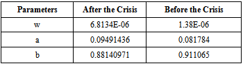
Table 3. ARCH(1,1) Parameters Before and After the Crisis
 |
| |
|
3.3. Comparison of Results: Before and After the Crisis
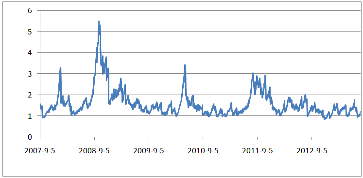 | Figure 1. Daily Volatility of Paris Bourse, September 3,2007-August 1, 2013 |
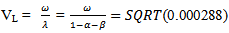
The same process was implemented for the period January 2001-March 2007. A significant difference in the daily volatility was observed over the two-period study. The highest volatility rate was 3.5% compared to 5.48% after the crisis. The long term volatility rate, VL, based on λ and  attained 1.39% compared to 1.69%. Table 3 depicts the difference in ARCH(1,1) parameters between both periods.
4. Discussion and Conclusions
The purpose of this paper being the parameterization of GARCH(1,1) for Paris Bourse cannot be achieved without proving the efficiency of this model as constituting a good tool for managing risks. As previously mentioned, the assumption underlying a GARCH model is that volatility changes with the passage of time. Therefore, an efficient GARCH model should remove the autocorrelation among the  . To this end we tested the autocorrelation structure for the variables
  . These showed very little autocorrelation[10], almost close to an average of 0.011 with each lag of time, and always much smaller in magnitude than the autocorrelation for
  . Therefore our procedure to accurately assess the Paris Stock Market volatility has succeeded and appeared to have correctly explained the volatility before and after the crisis. In the above described model we did not use the variance targeting approach, which is also a robust approach to estimating the GARCH(1,1) parameters. We will implement it in this section to confirm the GARCH(1,1) output. To this end we set VL equal to the median (1.41%) since we believe that such value is reasonable for after the crisis period, and then deduce the value of
  . Therefore only two parameters, α and β, are left to be estimated. The optimal values turn out to be 0.0863 and 0.92318 for α and β respectively. The value of the objective function is 11,143.662, slightly below the value of 11,176.60621 obtained using the earlier procedure. On the other hand, using EWMA model, where the procedure is simple[11], produced a value of λ = 0.939 that maximizes the objective function at a value of 10,780.392. This value of λ is very close to that used by the RiskMetrics database created by J.P. Morgan. We therefore conclude that the estimated parameters in GARCH(1,1) for Paris Bourse using the maximum likelihood methods succeeded to properly assess the volatility of this market after the 2007 financial crisis. However we do not pretend that GARCH(1,1) is the best model to be used by risk managers. We did use it because it simply corresponds to a simple news impact curve (before and after the crisis) which is the purpose of this study, although it is unable to generate a leverage effect. So far there are no much evidence that GARCH(1,1) model is outperformed because it is enough flexible to capture the persistence of volatility.
Notes
1. Considering that inflation uncertainty changes over time.2. The expected change in one day is very small when compared to the standard deviation of changes.3. If we substitute for  in equation (5), the estimate
  of the volatility for day n is therefore
  which is equal to
  . In a similar way when we substitute for
 we get
 .4. Where
  .5. As per the RiskMetrics database created by J.P. Morgan. 6. ui = (Si-Si-1)/Si-17. We made sure when we developed the spreadsheet model to relate all the variables with the appropriate cell formulas that relate the changing cells to the objective cell and formulas. 8.
 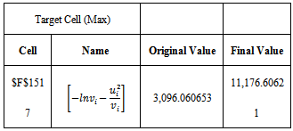 9.
9.  10. The Ljung-Box statistic can be use to perform the autocorrelation test. 11. Where
  and α = 1-λ, and β = λ and only one parameters has to be estimated.
References
| [1] | Bollerslev T. 1986. Generalized autoregressive conditional heteroskedasticity. Journal of Econometrics 31:309–328. |
| [2] | Engle R.F and Mezrich J. 1996. GARCH for Groups. Risk: 36-40. |
| [3] | Engle RF, Bollerslev T. 1986. Modelling the persistence of conditional variances. Econometrics Review 5: 1–50. |
| [4] | Engle RF, Gonzalez Rivera G. 1991. Semiparametric GARCH models. Journal of Business & Economic Statistics 9(4): 345–359. |
| [5] | Engle RF, Ito T, Lin W-L. 1990. Meteor showers or heat waves? Heteroskedastic intra-daily volatility in the foreign exchange market. Econometrica. 58(3): 525–542. |
| [6] | Engle RF. 1982. Autoregressive conditional heteroscedasticity with estimates of the variance of United Kingdom inflation. Econometrica 50(4): 987–1007. |
| [7] | Engle, R.F. and D. Kraft, 1983. Multiperiod forecast error variances of inflation estimated from ARCH models, in: A. ZeUner, ed., Applied time series analysis of economic data (Bureau of the Census, Washington, DC) 293-302. |
| [8] | Engle, R.F., 1983, Estimates of the variance of U.S. inflation based on the ARCH model, Journal of Money Credit and Banking 15, 286-301. |
| [9] | Engle, R.F., D. Lilien and R. Robins, 1985, Estimation of time varying risk premiums in the term structure, Discussion paper 85-17 (University of California, San Diego, CA). |
| [10] | Hansen R. and A. Lunde 2001. A comparison of volatility models: Does anything beat a GARCH(1,1) ? Working Paper Series No. 84. CAF, AArhus School of Business. |
 Abstract
 Reference
 Full-Text PDF
 Full-text HTML