Swarnima Bahadur, K. K. Mathur
Department of Mathematics & Astronomy, University of Lucknow, Lucknow, India
Correspondence to: Swarnima Bahadur, Department of Mathematics & Astronomy, University of Lucknow, Lucknow, India.
| Email: |  |
Copyright © 2012 Scientific & Academic Publishing. All Rights Reserved.
Abstract
Let (1) z0 = 1, z2n+1 = –1, zk = cos θk + i sin θk, zn+k = –zk, k = 1(1)2n be the vertical projections on unit circle of the zeros of (1 – x2)Pn(x), where Pn(x) stands for nth Legendre polynomial having the zeros xk = cos θk k = 1(1)n, such that 1 > x1 > … > xn > –1; Xie Siqing claimed regularity, explicit representation and convergence of (0, 1, 3) interpolation on the nodes (1). The explicit forms of these polynomials are very complicated as such in this paper, we obtain regularity, simpler explicit forms and quantitative estimate resulting convergence in the case of the weighted (0, 1, 3)–interpolation problem .
Keywords:
Legendre Polynomial, Explicit Representation, Convergence
Cite this paper: Swarnima Bahadur, K. K. Mathur, Weighted (0, 1, 3)* – Interpolation on Unit Circle, American Journal of Mathematics and Statistics, Vol. 3 No. 6, 2013, pp. 337-345. doi: 10.5923/j.ajms.20130306.06.
1. Introduction
In a paper Xie Siqing[6] considered vertical projections of the zeros of (1–x2)  , n even or (1 ± x)
  , n odd; on unit circle and established regularity of (0, 1, …, r – 2, r) – interpolation under certain restrictions on parameters α and β. In another paper[7], considering a particular case for r = 3 and assuming the nodes as :
 | (1.1) |
to be the vertical projections on unit circle of the zeros of (1–x2)Pn(x), where Pn(x) stands for nth Legendre polynomial having the zeros xk = cos θk. k = 1(1)n, such that 1 > x1 > x2 > … > xn> –1, Xie Siqing claimed regularity, explicit representation and convergence of (0, 1, 3)–interpolation viz. Rn(z) of degree ≤ 6n + 3 on the nodes (1.1) satisfying the conditions : | (1.2) |
where αpk,p = 0,1,3 are arbitrary given complex numbers. The explicit forms of these polynomials are very complicated as such in the last set of conditions (1.2) instead of prescribing  , we prescribe
  , k = 1(1)2n, which give simpler forms of the polynomials.On the suggestion of P. Turán, J. Balázs[1] for the first time investigated weighted (0,2)–interpolation taking nodes on the real line in[–1.1]. Later on L. Szili[5], K.K. Mathur and R.B. Saxena[3] extended the study of weighted (0,2) and weighted (0,1,3) –interpolations respectively on infinite interval (–∞, ∞).Weighted lacunary interpolatory problems on unit circle have not been considered on the literature so far, so the object of this paper is to obtain regulatory, explicit representation in a simpler form and a quantitative estimate leading to a convergence theorem in the case of weighted (0,1,3)–interpolation choosing special nodes on unit circles. The authors[4] have also made similar study in the case of weighted (0,2)–interpolation on unit circle.
2. Preliminaries
Let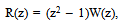 | (2.1) |
and | (2.2) |
where Pn stands for nth Legendre Polynomial and In the well known differential equation :
 | (2.3) |
taking  , we get
 | (2.4) |
Further owing to (2.1), (2.4) reduces to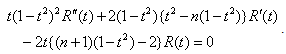 | (2.5) |
Also for k = 1(1)n, we have | (2.6) |
 | (2.7) |
and for k = 1(1)2n, we have | (2.8) |
The fundamental functions of Lagrange interpolation based on the nodes as zeros of W(z) and R(z) respectively are given by | (2.9) |
and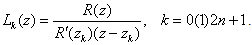 | (2.10) |
With the help of (2.2) and (2.9), we define Jk as | (2.11) |
 | (2.12) |
 | (2.13) |
For –1 ≤ x ≤ 1, we have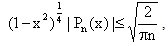 | (2.14) |
 | (2.15) |
 | (2.16) |
 | (2.17) |
Let xk's be the zeros of Pn(x), then | (2.18) |
 | (2.19) |
For –1 < x < 1, we have | (2.20) |
where c is a constant and
3. Regularity Ahd Explicit Representation of Interpolatory Polynomials
Let zk's be given by (1.1). We seek to determine the regularity of the polynomials Rn(z) of degree ≤ 6n+3, satisfying the conditions : | (3.1) |
where α0k, α1k and β3k’s are given arbitrary complex numbers. We call such polynomials as weighted (0,1,3)–interpolation on unit circle.Theorem 1 : In (3.1) if α0k = α1k = 0 for k = 0(1)2n + 1 and β3k = 0 for k = 1(1)2n, then Rn(z)=0.Proof: Since Rn(z) is a polynomial of degree at most 6n+3, we have Rn(z)=W(z)R(z)q(z), where W(z) and R(z) are given by (2.1) and (2.2) respectively and q(z) is a polynomial of degree at most 2n+1. Using the conditions (3.1), we get q’ (zk) = 0. Therefore, we may suppose q(z)=aJ0(z)+b, where a and b are constants and J0(z) is given in (2.11). Now, applying  ,we get q(z)=0,leading to Rn(z)=0, which completes the proof of the theorem.We write Rn(z) satisfying conditions (3.1) as
  | (3.2) |
where Ajk (j = 0,1,3) are unique polynomials each of degree ≤ 6n + 3 determined by the following requirements : | (3.3) |
 | (3.4) |
 | (3.5) |
Theorem 2 : Let R(z), W(z) and Jk(z) be given by (2.1), (2.2) and (2.11), then under conditions (3.5), A3k(z) are given  | (3.6) |
where | (3.7) |
 | (3.8) |
and | (3.9) |
Theorem 3 : Let Lk(z) and Hk(z) be given by (2.10) and (2.12), then under the conditions (3.4), A1k(z) is given by : | (3.10) |
where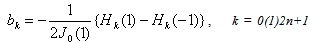 | (3.11) |
 | (3.12) |
 | (3.13) |
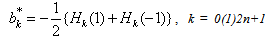
 Theorem 4 : Let L1k(z), Sk(z), A3k(z) and A1k(z) be given by (2.9), (2.13), (3.6) and (3.10), then under the conditions (3.3), A0k(z) is given by :
 | (3.14) |
where | (3.15) |
 | (3.16) |
 | (3.17) |
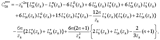 | (3.18) |
k = 1(1)2nProof of Theorem 2: Let A3k (z) be in (3.6). Obviously A3k(zj) = 0 for j = 0(1)2n+1 and A3k’ (zj) = 0 for j = 1(1)2n. From  ; j, k = 1(1)2n, we have
  . For
. For , result is obvious and for j=k, we get
  given in (3.7).Now, from the conditions
  , we get
  and
and  as given in (3.8) and (3.9),which proves the theorem.One can prove theorems 3 and 4 owing to conditions (3.4) and (3.5) respectively, so we omit the details of proof.
4. Estimation of Fundamental Polynomials
Lemma 1 : Let L1k(z) be given by (2.9), then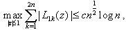 | (4.1) |
where c is a constant independent of n and z.Proof : Let z = x + iy and |z| = 1, then from (2.6) and (2.9), for 0 ≤ arg z < π and k = 1(1)n, one can see that 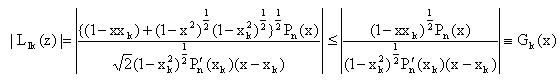 | (4.2) |
Also, | (4.3) |
Similarly, for π ≤ arg z < 2π and k = 1(1)n | (4.4) |
Therefore, for a fixed z = x + iy, |z| = 1 and |z| = 1 and –1 < x < 1, we have  | (4.5) |
Now,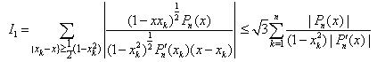 Using (2.16), (2.18) and (2.19), we get
 | (4.6) |
Further for –1 < x < 1, we have | (4.7) |
(4.5) with the help of (4.6) and (4.7) proves the lemma.Lemma 2 : Let J0(z) be given by (2.11), then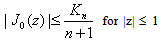 | (4.8) |
and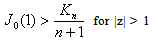 | (4.9) |
where Kn is defined by (2.2).Proof : To prove (4.8), we see that because of (2.16).Again
  using (2.17), we get the result.Lemma 3 : Let A3k(z) be given by (3.6), then
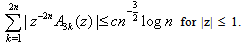 | (4.10) |
Proof : It is sufficient if we prove the lemma to be true for |z| = 1. Let z = eiα (0 ≤ α < 2π). From (3.6), we see that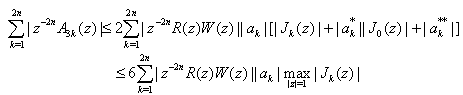 | (4.11) |
because from (3.8), lemma 2 and (3.9), one can see that From (3.7) and (2.6), we have
 | (4.12) |
From (4.11), (4.12) and | (4.13) |
 owing to (2.1), (2.2) and (2.14), we have
 From (2.18) and (2.19), we have
 which proves (4.10) owing to lemma 1.Lemma 4 : Let Hk(z) be given by (2.12), thenProof : The estimate of |Hk(z)|, for k = 0, 2n+1 follow from (2.12) and (4.8), so we omit the details.For estimate of
  , from (2.10), we have
 , for k = 1(1)2n.On further differentiating and rearranging terms, we get
 .From (2.12), we obtain
 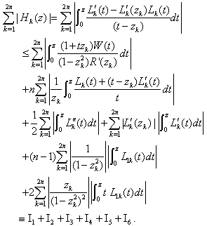 | (4.15) |
A little computation yields | (4.16) |
 | (4.17) |
and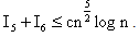 | (4.18) |
From (4.15) – (4.18) follows the lemma.Lemma 5 : For |z| ≤ 1, we have | (4.19) |
where A1k(z) is given by (3.10).Proof : Considering (3.10), we have | (4.20) |


 .From maximal principle, we have
 | (4.21) |
From (3.11), (3.12) and Lemma 2, | (4.22) |
Now, for the estimation of  , we have
 Using (4.13), (4.14) and (4.21), we get
 | (4.23) |
Similarly, one can have | (4.24) |
Further, we have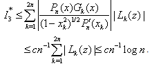 | (4.25) |
From (4.22), (4.13) and (4.14), we get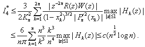 | (4.26) |
From (3.13), we have .Using this estimate and lemma 3, we get
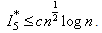 | (4.27) |
Thus, (4.20) owing to (4.23)–(4.27) complete the proof of the lemma. Lemma 6 : Let Sk(z) be given by (2.13), then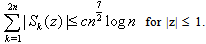 | (4.28) |
Proof : Let  ,
, | (4.29) |
and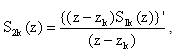 | (4.30) |
then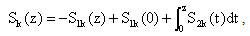 | (4.31) |
where Sk(z) is given by (2.13).Using (4.29) and Lemma 4, one can see that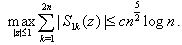 | (4.32) |
Similarly, we have | (4.33) |
Finally, the lemma follows from (4.31) – (4.33).Lemma 7 : For |z| ≤ 1, we have | (4.34) |
The proof of the lemma is similar to that of Lemma 5, so we omit the details.
5. Quantitative Estimate and Convergence Problem
In this section, we shall prove the following :Theorem 4 : Let f(z) be continuous in the region |z| ≤ 1 and analytic in |z| < 1, then the sequence {Rn} defined by | (5.1) |
satisfies the relation : | (5.2) |
where c is independent of n and z, ω2(f,δ) is the modulus of smoothness of f(z).Remark : Let f(z) be continuous in |z| ≤ 1 and f '∈Lip. α, α > ½, then the sequence {Rn} converges uniformly to f(z) in |z| ≤ 1, which follows from (5.2) and .To prove theorem 4, we need the following well known Jackson’s theorem :Let f(z) be continuous in the region |z| ≤ 1 and analytic in |z| < 1, then there exists a polynomial Fn(z) of degree ≤ 2n – 2 such that
 | (5.3) |
where z = eiθ, 0 < θ ≤ 2π.To prove our theorem, we shall also require | (5.4) |
which is an easy consequence of an inequality of ), Kis[[2],[32]] viz. , m = 0, 1, …. and
 Proof of the main Theorem 4 : Since Rn(z) given by (3.2) is a uniquely determined polynomial of degree ≤ 6n + 3, therefore, the polynomial Fn(z) satisfying (5.3) and (5.4) can be expressed as
  Then
Then  Taking z = eiθ, 0 < θ ≤ 2π and using (5.3), (5.4), Lemma 3, Lemma 5 and Lemma 7, we get (5.2) which completes the proof of the theorem.
References
| [1] | J. Balázs, Sulyozott (0,2)–interpolacio ultraszferikus polinomok gyokein, MTA III, Oszt. Kozl., 11(1961), 305–338. |
| [2] | O.Kiś, Remarks on interpolation (Russian), Acta Math. Acad. Sci. Hungar. 11(1960), 49–64. |
| [3] | Mathur, K.K. and Saxena, R.B., Weighted (0,1,3) –interpolation on the zeros of Hermite polynomials, Acta Math. Hung., 62(1–2)(1993),32–47. |
| [4] | Mathur, K.K. and Bahadur, S., Weighted (0,2)–interpolation on unit circle , Int. J. Appl. Math. Stat., Vol. 20,M 11, 2011. |
| [5] | Szili, L., Weighted (0,2)–interpolation on the roots of Hermite polynomial, Ann. Univ. Sci., Budapest Eötvös Sect Math, 27(1984), 153–166. |
| [6] | Xie, Siqing, Regularity of (0,1,…, r–2, r) and (0,1,…, r–2, r)*–interpolation on some sets of the unit circle, J. of Approx. Theory, 1995, 82(1), 54–59. |
| [7] | Xie, Siqing, Convergence of (0,1,3)*–interpolation on unit circle, Acta Mathematic Sinica, 1996, 39(5), 690–700. |
 Abstract
 Reference
 Full-Text PDF
 Full-text HTML