-
Paper Information
- Next Paper
- Paper Submission
-
Journal Information
- About This Journal
- Editorial Board
- Current Issue
- Archive
- Author Guidelines
- Contact Us
American Journal of Mathematics and Statistics
p-ISSN: 2162-948X e-ISSN: 2162-8475
2013; 3(6): 315-331
doi:10.5923/j.ajms.20130306.04
Heteroscedastic Analysis of the Volatility of StockReturns in Nairobi Securities Exchange
 Abstract
 Reference
 Full-Text PDF
 Full-text HTML
MutaiCheruiyot Noah, Mung’atu Kyalo Joseph, Waititu Gichuhi Anthony
Jomo Kenyatta University of Agriculture and Technology, Nairobi, Kenya
Correspondence to: MutaiCheruiyot Noah, Jomo Kenyatta University of Agriculture and Technology, Nairobi, Kenya.
| Email: |  |
Copyright © 2012 Scientific & Academic Publishing. All Rights Reserved.
Heteroscedasticity arises when the error term of a regression equation does not have a constant variance. Financial markets are known to be very uncertain a phenomenon called volatility which is a key variable used in many financial applications such as investment, portfolio construction, option pricing and hedging as well as market risk management. This study models the heteroscedasticity of volatility of stock returns in Nairobi Securities Exchange, NSE of Safaricom and Kenya Commercial Bank, KCB using daily return series from 9th June 2008, to 31st December, 2010, using ARIMA-ARCH/GARCH models. The procedure for building the model involved model identification, order determination, estimation of parameters and diagnostic check.Shapiro–Wilk testrejected the null hypothesis of normality for both series at 5% level of significance while Philip Perron (PP) and Augmented Dickey Fuller (ADF) reveal that price series were not stationary while returns series were stationary. All the return series exhibit, leptokurtosis, volatility clustering and negative skewness. The estimation results reveal that ARIMA (1, 0, 0)-GARCH (1, 1) and ARIMA (0, 0, 2)-GARCH (1, 1) best fits Safaricom and KCB respectively. Investors who wish to avoid large, erratic swings in portfolio returns may wish to structure their investments to produce a leptokurtic distribution. Further, researches should focus on the calculation of value-at-risk (VaR) in the markets.
Keywords: Heteroscedasticity, Volatility, Returns, ARIMA-GARCH-models
Cite this paper: MutaiCheruiyot Noah, Mung’atu Kyalo Joseph, Waititu Gichuhi Anthony, Heteroscedastic Analysis of the Volatility of StockReturns in Nairobi Securities Exchange, American Journal of Mathematics and Statistics, Vol. 3 No. 6, 2013, pp. 315-331. doi: 10.5923/j.ajms.20130306.04.
Article Outline
1. Introduction
- In recent years, modeling and analyzing stock return volatility is one of the most important aspects of financial market developments, providing an important input for portfolio management, option pricing and market regulation [1]. An investor’s choice of a portfolio is intended to maximize the expected return subject to a risk constraint, or to minimize his risk subject to a return constraint. An efficient model for forecasting of an asset’s price volatility provides a starting point for the assessment of investment risk. To price an option, one needs to know the volatility of the underlying asset. This can only be achieved through modeling the volatility. Volatility also has a great effect on the macro-economy. High volatility beyond a certain threshold will increase the risk of investor loses and raise concerns about the stability of the market and the wider economy[2].In Kenya and other countries, investing in stocks has attracted many individuals. This can be evidenced by the number of people who showed interest in buying the Safaricom IPO’s during its inception in 2008. Returns from these stocks tend to fluctuate over time. They are thus volatile and exhibit volatility clustering. Due to the exponential growth in those investing in stocks, modeling and analyzing volatility of stock market returns has become an important research area in financial markets and has received much attention from market practitioners, analysts and organizations with the aim of coming up with robust models that can predict future prices. This extensive research reflects the importance of volatility in investment, security valuation, risk management and monetary policy making[1]Both academicians and practitioners recognize that volatility is not directly observable and that financial returns show certain characteristics that are specific to financial time series such as volatility clustering and leverage effect[3]. Financial econometricians have developed manytime-varying volatility models among them, the Autoregressive Conditional Heteroscedastic(ARCH) model proposed by Engle[4] and its extension, the Generalized Autoregressive Conditional Heteroscedastic(GARCH) developed by Bollerslev[3], and Taylor[5] which have been applied widely. This research seeks to investigate the dynamics of stock return volatility in NSE. This is due to the growth in those investing in stocks in Kenya and it has become one way of building wealth. Investors normally anticipate for high returns but are also aware of the risk involved due to fluctuation in prices.
2. Literature Review
- Financial time series modeling has been a subject of considerable research both in theoretical and empirical statistics and econometrics. Various linear and non-linear methods by which such forecasts can be achieved have been developed in the literature and extensively applied in practice to describe stock return volatility. Such techniques range from linear to non-linear models. Poterba[6] take into account the linear model and specify a stationary AR (1) process for volatility of the S&P 500 index. Another study by Frenchet al[7] uses a non-linear stationary ARIMA (0, 1, 3) model to describe the volatility of the S&P 500 index. The extensive use of such models is not surprising since they provide good first order approximation to many processes. Linear time series models however are not robust to describe certain features of a volatility series. For instance there are well-defined empirical evidences that stock returns have a tendency to exhibit clusters of outliers, implying that large variances tend to be followed by another large variance. They are unable to explain a number of important features common to much financial data, including leptokurtosis, volatility clustering, long memory, volatility smile and leverage effects. That is, because the assumption of homoscedasticity (or constant variance) is not appropriate when using financial data, and in such instances it is preferable to examine patterns that allow the variance to depend upon its history. Thus such limitations of linear models have motivated many researchers to consider non-linear alternatives. The Autoregressive Conditional Heteroscedastic (ARCH) model of Engle[3], the generalized ARCH (GARCH) model of Bollerslev[3] and exponential GARCH (EGARCH) model of Nelson[8] are the common non-linear models used in finance literature. These ARCH class models have been found to be useful in capturing certain non-linear features of financial time series such as heavy tailed distributions and clusters of outliers. A study by Akgiray[9] uses a GARCH(1,1) model to investigate the time series properties of the stock returns and reports GARCH to be the best of several models in describing and forecasting stock market volatility. Anil & Higgins[10] investigated the volatility of the conventional ordinary least squares to estimate optimal hedge ratio estimates using future contracts. Similarly, Najand[11] examines the relative ability of linear and non-linear models to forecast daily S&P 500 futures index volatility. The study finds that non-linear GARCH models perform best. Benoit [12] utilized the infinite variance distributions, when considering the models for stock market price changes. Fama[13] when modeling stock market prices attributed their discrepancies to the possibility of the process having stable innovations and thus fitted an adequate model on this basis. Markov-Switching models have also been used to capture the volatility dynamics of financial time series. This is because they give rise to a plausible interpretation of nonlinearities. Markov switching model of stock returns was originally proposed by M, Startz, & Nelson[14]. Bhar[15], among others employ markov switching models for the modeling of stock returns. There is a significant amount of research on volatility of stock markets of developed countries. For instance, Gary[16] applied the GARCH model to the Shanghai Stock Exchange while Bertram[17] modeled Australian Stock Exchange using ARCH models. Other studies on these stock markets include Baudouhat[18] who utilized the GARCH model in analyzing the Nordic financial market integration. Walter [19] applied the structural GARCH model to portfolio risk management for the South African equity market as well Hongyu[2] who forecasted the volatility of the Chinese stock market using the GARCH-type models. Elie[20] compared the GARCH model and the EGARCH under three distribution assumptions: the Gaussian, the t-student and the general error distributions. He showed that the distribution of returns is far from being normally distributed with fat tails and volatility clustering being persistent. Al-Jafari[21] utilized a non-linear symmetric GARCH(1,1) model and two non-linear asymmetric models, TARCH(1,1) and EGARCH (1,1) to Muscat Securities Market and the empirical findings provide no presence of day-of –the –week effectThe Sub-Saharan Africa has been under-researched as far as volatility modeling is concerned. Studies carried out in the African stock markets include, Frimpong Joseph Magnus [22] who applied GARCH models to the Ghana Stock Exchange. Brooks[23] examined the effect of political change in the South African Stock Market;Appiah-Kusi[24] investigated the volatility and volatility spillovers in the emerging markets in Africa. More recently, Emenike[25] applied the EGARCH model to the Kenyan and Nigerian Stock Market returns. From the available literature, the NSE just like other Sub Saharan Africa Equity Markets has been under-researched as far as market volatility is concerned and therefore this study contributes to the small literature available on the Nairobi stock market.These developments in financial econometrics suggest the use of nonlinear time series structures to model the stock market prices and the expected returns. The focus of financial time series modeling has been on the ARCH model and its various extensions. However, the ARCH has limitations in that it treats negative and positive returns in the same way. It is also very restrictive in parameters and often over predicts the volatility because it responds slowly to large shocks. GARCH models have proved adequate in modeling and forecasting volatility. GARCH for instance takes into account excess kurtosis i.e. fat tail behavior and volatility clustering which are two important characteristics if time series. It also provides accurate forecast of variances and covariance of asset return through its ability to model time varying conditional variances. However, GARCH is only part of a solution. Although GARCH models are usually applied in return series financial decisions are rarely based solely on expected returns and volatilities. GARCH models are parametric specifications that operate best under relatively stable market conditions. Also GARCH is explicitly designed to model time-varying conditional variances. GARCH models often fail to capture highly irregular phenomenon. These include rebounds and other highly anticipated events that can lead to significant structural change. Further, GARCH models fail to capture the fat tails observed in asset return series. Some scholars favor Markov-Switching models claiming that; Markov- Switching models are more accurate and provide better forecasts than a variety of linear and non-linear GARCH models for instance[14]. In this paper we use ARIMA- ARCH/GARCH models of stock returns to model the heteroscedastic nature of volatility of stock returns in the Nairobi stock market over the period June 6, 2008 to December 31, 2010.
3. Materials and Methods
3.1. Materials
3.1.1. Data for the Study
- The data used in this study comprise Safaricom’s and KCB’s daily returns series over the period June 6, 2008 to December 31, 2010. The closing prices were obtained fromNairobi Securities Exchange. Since the return of an asset is a complete and scale free summary of an investment with attractive statistical features, we used return series rather than the price series[26].
3.2. Methods
3.2.1. Volatility Definition and Measurement
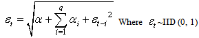
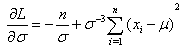
- Volatility refers to the fluctuation observed in some phenomenon over time. In modeling and forecasting literature it refers to the conditional variance of the underlying asset return. It is measured as the sample standard deviation;
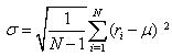 | (1) |
 is the standard deviation,
  is the return on day i and
  is the average return over the N-day period
3.2.2. Basic Statistics of Returns
3.2.2.1. Descriptive Statistics
- Analyzing financial prices directly is difficult because consecutive prices are correlated, and the variances of prices frequently increase with time. Consequently we use price changes to analyze prices. There are two main types of price changes that are used: arithmetic and geometric returns.[27]Definition: Let
 and
and  be today’s and yesterday’s prices of an asset or a portfolio, the arithmetic returns are defined by
 | (2) |
 is the price of the asset at day t. Yearly arithmetic returns are defined by:
 | (3) |
 and
and  are the prices of the asset at the first and the last trading day of the year, respectively. Then, R may be written as
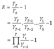 | (4) |
 and
and  be today’s and yesterday’s prices of an asset or portfolio, then the geometric returns are defined as
 | (5) |
 | (6) |
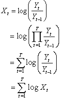 | (7) |
3.2.3. The Normality Test
- This tests the likelihood that the given data set
 comes from a Gaussian distribution. A great number of tests have been devised for this problem. One of the tests used is the Shapiro–Wilk test. In statistics, the Shapiro–Wilk test tests the null hypothesis that a sample
  came from a normally distributed population. It was published in 1965 by Samuel Shapiro and Martin Wilk. The test statistic is:
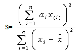 | (8) |
 with parentheses enclosing the subscript index (i) is the
  order statistic, i.e., the
  -smallest number in the sample;ii)
  is the sample mean;iii) the constants
  are given by
 | (9) |
 are the expected values of the order statistics of independent and identically-distributed random variables sampled from the standard normal distribution, and V is the covariance matrix of those order statistics.
3.2.4. Volatility Clustering
- This is determined by computing the ACF. Given that
 is a stationary time series, with constant expectation and time independent covariance. The ACF for the series is defined as
 | (10) |
 and
and  The value k denotes the lag.Plots of ACF as a function of k shall be done, and determine if the autocorrelation decreases as the lag gets larger or of if there is any particular lag for which the autocorrelation is large
3.2.5. Testing for ARCH Effects
- Before fitting the autoregressive models to each of the daily returns series, the presence of ARCH effects in the residuals is first tested. If there does not exist a significant ARCH effect in the residuals then the ARCH model is mis-specified. Testing the hypothesis of no significant ARCH effects is based on the Lagragian Multiplier (LM) approach, where the test statistic is given by
 | (11) |
 =the coefficient of determination for the regression in the ARCH model using the residuals. The null hypothesis is that there is no ARCH effect up to order
  in the residuals. The test statistic is calculated as the number of observations multiplied by
  from the regression. The LM test statistic asymptotically follows a
  distribution. The null hypothesis is rejected if the test statistic is larger than critical value of
3.2.6. Testing for Stationarity and Autocorrelation
- Test for stationarity is conducted with the Augmented Dickey Fuller (ADF) and Philip Perron (PP) test. The null hypothesis is that the return series have unit roots or in other words, the series is non-stationary. The null hypothesis is rejected if the test statistic is larger in the absolute term than the critical value[28]Having confirmed that all return series are stationary, we shall continue to examine the autocorrelation and the partial autocorrelation in the series to identify their proper structures. This is done through the Ljung-Box Q-statistic test by (Box & George[29] which is defined as:
 | (12) |
 is the sample autocorrelation coefficient; T is the sample size and m is the maximum lag lengthThe null hypothesis that all
  are zerois rejected if the value of the computed Q is larger than the critical Q-statistic from the chi-square distribution at the given level of significance. According to Harvey & Jaeger[30], choosing the number of lags for the test is a practical issueas a small number of lags might fail to detect the autocorrelations at high-order lags, whereas, a large number of lags might result in diluting the significant correlation at one lag by insignificant correlations at other lags.
 3.2.7. Volatility Modeling Techniques
3.2.7.1. ARCH Model
- The ARCH model was introduced by Engle[4] in his study “Autoregressive Conditional Heteroscedasticity with estimates of the Variance of United Kingdom Inflation”, as the first formal model which seemed to capture the phenomena of changing variance in time series data. It is most widely used discrete time model for analysis of financial data. The formulation of his model is given below:
 | (13) |
 where
where  is the variance at time t,
  is square residuals at rime t, and q is the number of lags. The effect of a return shock i period ago (i≤ q) on current volatility is governed by the parameter α. In an ARCH model, old news arrived at the market more than q period ago has no effect at all on current volatility. For ARCH (1, 1) the model is
3.2.7.2. GARCH Model
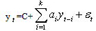
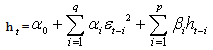
- Bollerslev[3] extended the basic ARCH model by introducing the GARCH model which has proven to be quite useful in empirical work. He suggested that the conditional variance function be specified as follows:

 is the mean equation. Where
  is the stock return,
  is the exogenous variables or belonging to the set of information
  , β is a fixed parameter vector and conditional variance is,
 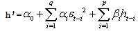 | (14) |
 and
and 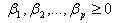 The GARCH (p, q) above defined as stationary when
  . In this study we are going to use GARCH (1, 1). The model for GARCH (1, 1) is given by
 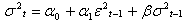 where,
  and
and 
3.2.8. Building a Volatility Model
3.2.8.1. Model Identification
- Under the identification stage the following wasdone: i. Converting of daily closing price series to return series. Let
 denote the daily closing price of a stock at the end of the day t, the daily stock return series is generated by
  | (15) |
 the LM test statistic equal to
  has asymptotic chi -squared distribution with p degree of freedom.iii. An ARIMA(p,d,q) model was fitted to the data to remove serial dependenceiv. ACF, PACF and AICc was used to determine the order of the models
3.2.8.2. Parameter Estimation
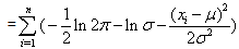
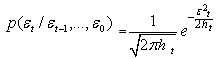
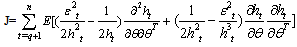
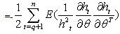
- The estimation of the model’s parameters was implemented by Maximum Likelihood Method under the normal distribution. This involves choosing values for the parameters that maximizes the chance (or likelihood) of the data occurring. Given a sample
 of n, IID observations, which comes from a distribution f(x) with unknown parameter
  , then; the joint density function is
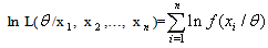
 | (16) |
 to be fixed parameters of this function, whereas
  will be the function's variable and allowed to vary freely. And this function is called likelihood
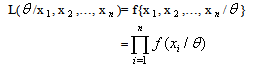 | (17) |
 | (18) |
 follow normal distribution with un-known parameters
  then
then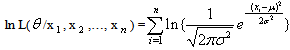 | (19) |
 | (20) |
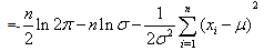 | (21) |
 and
and  as the un-known parameters
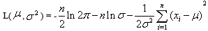 | (22) |
 | (23) |
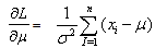
 | (24) |
 and
and  gives
gives | (25) |
 | (26) |
 | (27) |
 | (28) |
 | (29) |
 is the white noise term,
  is normally distributed with mean zero and variance
 | (30) |
 (
( becomes
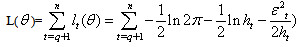 | (31) |
 | (33) |
 | (34) |
 | (35) |
 | (36) |
 | (37) |
3.2.8.3. Diagnostic Checking
- Goodness-of-fit needs to be performed after fitting the appropriate model Tackle[31]. This is based on the standardized residuals. The following was performed:i. The standardized residuals of the fitted model are analyzed to ascertain their randomness. The standardized residuals
 | (38) |
 nor
nor  should exhibit serial correlation.ii. The normal plots, ACF plot and time series plot was done. The normal probability plot should be a straight line while the time plot should exhibit random variation. For ACF’s all the correlation should be within the test bounds which indicates stationarity in the data.iii. Ljung-Box test is employed to check for adequacy of the fitted model. The Ljung-Box test was named after Greta M Ljung and George E. P. It is a type of statistical test which test whether any of a group of autocorrelations of a time series is different from zero. It performs a lack-of-fit hypothesis test for model specification, which is based on the Q-statistic
 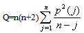 | (39) |
 is the squares sample autocorrelation at lag j. Under the null hypothesis of no serial correlation, the Q-statistic is asymptotically Chi-Square distributed. If the value of the test statistic is greater than the critical value from the Q-statistics, then the null hypothesis can be rejected. Alternatively, if p-value is smaller than the conventional significance level, the null hypothesis that there are no autocorrelation will be rejected.
 3.2.9. Volatility Forecasting
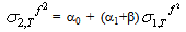
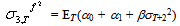
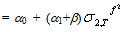
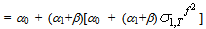
- The challenge in Econometrics is to specify how the information will be used to forecast the mean and variance of the return, conditional on the past information. Various methods have been considered for the mean return to forecast future returns. The most widely used specification is the GARCH (1, 1) model introduced by Bollerslev[3] as a generalization of Engle[4]. Consider the following GARCH (1, 1) model:
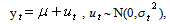 | (40) |
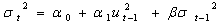 | (41) |
 | (42) |
 | (43) |
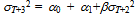 | (44) |
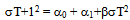
 be the one step ahead forecast for σ2 made at time T. This is easy to calculate since, at time T, the values of all the terms on the right hand side are known.
  , will be obtained by taking the conditional expectation of (40). Given
 ,
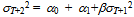
,  the 2-step ahead forecast for σ2 made at time T is obtained by taking the conditional expectation of (41)
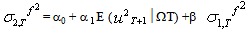 | (45) |
 is the expectation, made at time T, of
  , which is the squared disturbance term. We can write
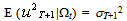 | (46) |
 , so that the 2-step ahead forecast is given by
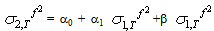 | (47) |
 | (48) |
 | (49) |
 | (50) |
 | (51) |
 | (52) |
 | (53) |
4. Results and Discussion
4.1. Data Exploration
- The data employed in this study comprise Safaricom’s and KCB’s closing price over the period June 6, 2008 to December 12, 2010 which constitutes a sample of 653 observations. The closing prices were obtained fromNairobi Securities Exchange. Let
 denote the daily closing price of a stock at the end of the day t, the daily stock return series was be generated by
 | (54) |
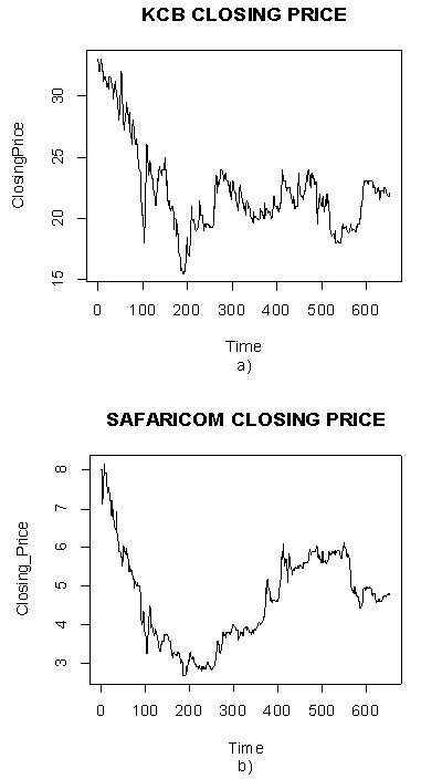 | Figure 1. Time series plot of KCB and Safaricom closing price |
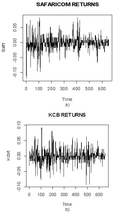 | Figure 2. Plots of Safaricom’s and KCB’s returns  |
4.1.1. Descriptive Statistics for the Prices and Returns
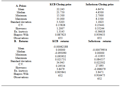
- Table 1 below shows summary statistics for the two companies’ return series. The results indicate high volatility and the risky nature of the market since the standard deviation of the market returns is high in comparison with the mean. Also the standard deviations are very close for both Safaricom and KCB with Safaricom being slightly volatile. Both price series have positive skewness implying that the distribution has a long right tail. On the other hand, the return series for Safaricom have negative skewness implying that the distribution has a long left tail and positive for KCB implying that the distribution has long right tail. The values for kurtosis are high (above three) for both return series implying they are leptokurtic. The Shapiro-Wilk test rejects normality at the 5% level for all series. So, the samples have all financial characteristics: volatility clustering and leptokurtosis.
|
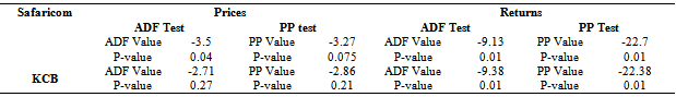
4.1.2. Test for Normality and Unit Root
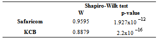
- Shapiro-Wilk test is used to test for normality in the series which are shown in the table below
|
|
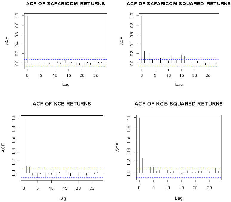 | Figure 3. ACF of Asset Returns and Squared Asset Returns for Safaricom and KCB |
4.2. ARIMA (p, d, q) Modeling
4.2.1. Model Identification
- Use ACF and PACF identify the ARIMA model for the mean equationThe upper left graphs show ACF of Log Safaricom closing price, showing the ACF slowly decreases. It is probably that the model needs differencing. The lower left is PACF of Log Safaricom closing price, indicating significant value at lag 1 and then PACF cuts off. Therefore, the model for Log Safaricom closing price might be ARIMA (1, 0, 0). The upper right shows ACF of differences of log Safaricom with no significant lags. The lower right is PACF of differences of log Safaricom, reflecting no significant lags. The model for differenced log Safaricom series is thus a white noise, and the original model resembles random walk model ARIMA (0, 1, 0)
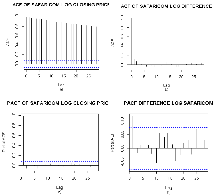 | Figure 4. ACF and PACF Safaricom closing and log differenced closing price |
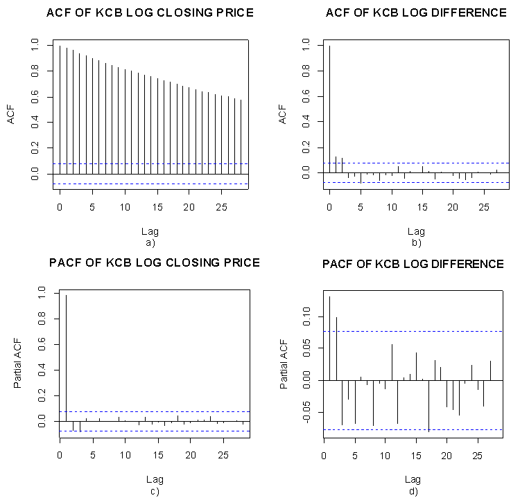 | Figure 5. ACF and PACF KCB closing and log differenced closing price |
|
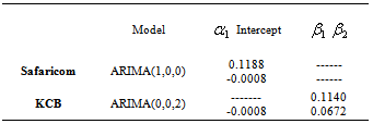
4.2.2. Parameter Estimation
- The parameters of the fitted ARIMA models are shown in the table below
|
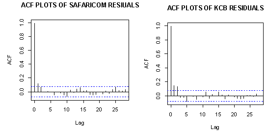
4.2.3. Diagnostic Checking
- We plot he ACF and the PACF of residuals to check for model adequacy.
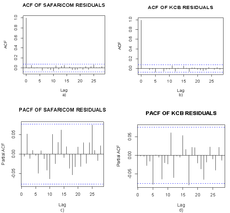 | Figure 6. ACF and PACF of Safaricom and KCB residuals |
4.3. ARCH/GARCH Modeling
- Although ACF & PACF of residuals have no significant lags, the time series plot of residuals shows some cluster of volatility (not reported here). ARIMA is a method to linearly model the data and the forecast width remains constant because the model does not reflect recent changes or incorporate new information. However, we fit an ARIMA (p, d, q) model to remove serial dependence in the series. Inspection of residual plot displays and squared residual plot shows cluster of volatility. The ACF & PACF of squared residuals confirms this and thus if the residuals (noise term) are not independent and can be predicted. Hence, ARCH/GARCH should be used to model the volatility of the series to reflect more recent changes and fluctuations in the series. Followings are the plots of squared residuals.
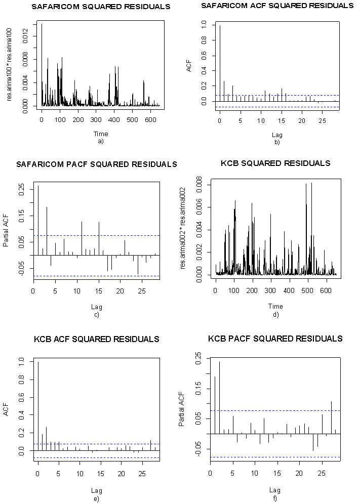 | Figure 7. ACF and PACF plots of residuals and squared residuals of Safaricom and KCB |
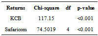
4.3.1. Testing for ARCH effects in Returns of  in the Fitted ARIMA (1,0,0) and ARIMA (0,0, 2)
- Before fitting the autoregressive models to each of the daily returns series, the presence of ARCH effects in the residuals is tested. If there does not exist a significant ARCH effect in the residuals then the ARCH model is mis-specified. Testing the hypothesis of no significant ARCH effects is based on the Lagragian Multiplier (LM) approach as stated earlier on the methodology.From Table 6, the p-values for both series are less than 0.05 hence we reject the null hypothesis of no significant arch effect in the daily returns of Safaricom and KCB and conclude there are significant arch effects for the June 6, 2008 to December 31, 2010.
|
4.3.2. Model Identification
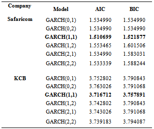
- Since this study deals with daily returns, it is restricted to pure ARCH (p) models. For GARCH (p, q) models, those with p, q ≤ 2 are typically selected by AIC and BIC. Low order GARCH (p, q) models are generally preferred to a high order ARCH(p) for reasons of parsimony and better numerical stability of estimation
4.3.3. Order Determination
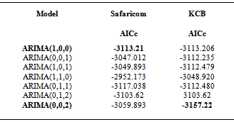
- Determining the ARCH order p and the GARCH order q for a particular series is an important practical problem. The AIC, BIC and Log likelihood ration tests are used in selecting the appropriate order of the GARCH from competing models. Table 7 below gives the suggested order with their respective fit statistics. The aim is to have a parsimonious model that captures as much variation in the data as possible. Usually the simple GARCH model captures most of the variability in most stabilized series. Small lags for p and q are common in applications. Typically GARCH (1, 1); GARCH (2, 1) or GARCH (1, 2) models are adequate for modeling volatilities even over long sample periods[33]. This study has included GARCH (1, 0) GARCH (0, 2) and GARCH (2, 2) in order to check if they are appropriate for modeling time varying variance. We select the model with the lowest AIC and BIC`From Table 7 above the model given in bold is taken to be the most appropriate according to the criteria above. The GARCH models for different values of p and q were fitted to the data, diagnosed and from the diagnosis and goodness of fit statistics, the GARCH (1, 1) was found to be the best choice. This is consistent with most empirical studies involving the application of GARCH models in financial time series data. We thus fit a GARCH (1; 1) to the residuals of ARIMA (1, 0, 0) and ARIMA (0, 0, 2) of Safaricom and KCB respectively.
|
4.3.4. Estimation
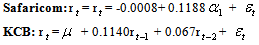
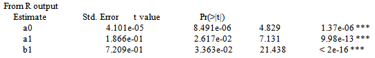 For Safaricom the fitted GARCH (1, 1) model is
 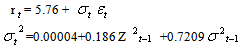 From the following output for KCB
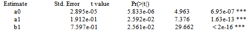 The fitted GARCH (1, 1) model is
 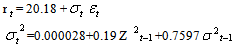 To assess the accuracy of the estimates, the standard errors are used the smaller the better. Model fit statistics used to assess how well the model fit the data are the AIC and BIC. From the standard errors the estimates are precise. Based on 95% confidence level, the coefficients of the fitted GARCH (1, 1) model are significantly different from zero.
4.3.5. Diagnostic Checking
- Here the adequacy of the selected models is done. This is done by using standardized residuals which are assumed to follow either normal or standardized t distribution. It must satisfy the requirement of a white noise. The plots include normal plots, ACF plot time series plot and histogram. If the model fits the data well the histogram of the residuals should be symmetric. The normal probability plot should be a straight line while the time plot should exhibit random variation. For ACF plots all the correlation should be within the boundary line meaning the data is stationary.
 | Figure 8. ACF plots of residuals for Safaricom and KCB |
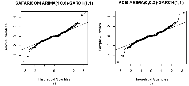 | Figure 9. Q-Q plots and Normal probability plot of Safaricom and KCB residuals |
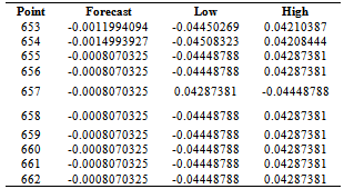
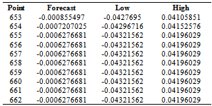
4.4. Volatility Forecasting
- The final objective of this study was to forecast the volatility. Table 8 and 9 below shows the forecastsAlthough forecast performance was not one of the objectives of the study, comparing GARCH(1,1) and mixed models using Mean Squared Error it was found that mixed models outperform GARCH(1,1)(results not presented here)
|
|
5. Conclusions and Suggestions
- The objectives of the study of this research work have been largely achieved. The return series of Safaricom and KCB series have been modeled. They reveal some stylized facts such as negative skewness, leptokurtosis, and volatility clustering, nonlinear data generating process, serial dependence and leverage effects which are common observations in other stock markets. This is agreement with previous researches. The null hypothesis of significant correlations is rejected at 5% level of significance for the two series. The results of LM test finds presence of arch effects and that the standardized residuals are normally distributed. It has been shown that the price is not normally distributed,which suggests that there is evidence of fat tails or is leptokurtic which is a common feature of financial market returns. Investors who wish to avoid large, erratic swings in portfolio returns may wish to structure their investments to produce a leptokurtic distribution.Other researchers can use heavy tailed distributions e.g General Error Distribution to capture the stylized facts of return series. Further, in emerging markets, diversification and return benefits provided have attracted significant investors’ interest which have led to significant portfolio equity inflows into these financial systems, and as a result, motivated the study of various aspects of stock return behavior in these markets. For that reason, an imperative and contemporary filament of empirical researches should focus on the calculation of value-at-risk (VaR) in the markets.