1. Introduction

Many different approaches such as Linear, Non-Linear, stochastic and non-stochastic models have been proposed in literature for the purpose of analyzing time series data. In recent years, the use of non-stochastic models has become widespread. Fuzzy time series forecasting models do not require assumptions that stochastic models do. On the other hand, most of the time series encountered in real life should be considered as fuzzy time series due to the uncertainty that they contain, also they should be analyzed with models appropriate to fuzzy set theory.

Chen[4] presented a simplified method of fuzzy time series forecasting of enrollments using arithmetic operations. Song and Chissom[22-24] used the fuzzy set theory given by Zadeh[28,29] to develop the time variant and time invariant models for fuzzy time series forecasting, and considered a problem of forecasting student enrollments on time series data of the University of Alabama.

A fuzzy time series method consists of three steps, those being fuzzification, identification of fuzzified relations and defuzzification, respectively. Many studies on these three steps have been done in literature because of these steps have either positive or negative impact on the forecastingperformance of the method. Some of the approaches proposed in the literature involve first-order forecasting models whereas some of them involve higher order forecasting models. Chen [4], Song and Chissom[22-24], Yolcu et al.,[27] can be given as examples of first-order fuzzy time series forecasting models. Also, Chen[5] and Aladag et.al.,[2] studies involve high-order fuzzy time series forecasting models.

Further, many researchers, Hwang[6], Huarng[9-10], Kim and Lee[11], Sullivan and Woodall[24], Tasi and Wu[25], worked on the development of various models of fuzzy time series forecasting and its implementations.

In the present work the proposed model was implemented on the historical Paddy crop yield forecast, which is a highly non-linear process, where data in general contains imprecision. The study is aimed to get some reliable forecast method for Paddy production during a lead year. This production forecast shall help the farmers as well as the local agro based industries in their process of business planning.

2. Materials and Methods

To achieve the stipulated objectives, the present study had been carried out on the basis of time-series production data of paddy crop pertaining to the period 1950-51 to 2009-10 had been collected through the Tamil Nadu government Agriculture Statistical office in Chennai, India. The main tools used were the nonlinear models were first checked for its appropriateness and then Fuzzy time series model approach and was concluded giving the best model that suited based on the lower values of Root Mean Square Error (RMSE), Mean Absolute Error (MAE), Mean Square Error (MSE) and Average Forecasting Error Rate (AFER )of the model.

2.1. Non-Linear Models

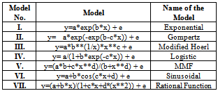
In parametric model different non-linear models given in table 1 (Bard[3], Draper and Smith[7], Montgomery[14], Ratkowsky[18], Seber and Wild[19]) were employed. Among the non-linear models, the model having highest adjusted R² with significant F value was selected, so that it satisfies test for goodness of fit (Montgomery[14]). Normality of residuals was examined by usingShaprio-Wilks test (Agostid’no and Stephens[1]). Further more, while dealing with time-series data it may be possible that successive observations may be auto correlated among themselves (Venugopalan and Shamasundaran[26]). To overcome all these problems, performing residual analysis is strongly advised. Randomness assumption of the residuals needs to be tested before taking any final decision about the adequacy of the model developed. To carry out the above analysis “Run test” procedure developed in the literature (Ratkowsky[18]). Further, to test the presence or absence of autocorrelation in the data set Durbin-Watson test procedure (Lewis-Beck[13]) is utilized In case of more than one model being the good fit for the data, the best model was selected having lower values of RMSE, MAE, MSE and AFER.

Table 1. List of non-linear models

In table 1, y is the production; x is the time points; a, b, c and d is the parameters; and e is the error term. In addition, a represents the carrying capacity, c is the intrinsic growth rate, b represents different functions of the initial value y(0) and d is the added parameters in the sinusoidal and rational function models.

The widely used Levenberg-Marquardt algorithm (Ratkowsky[18]) is utilized to fit the Modified Hoerl, Sinusoidal and rational function models. Different initial parameters values were used to ensure global convergence. The iterative procedure was stopped whenever the successive iterations parameter estimate values were negligible. The standard SPSS Ver. 10.1 package was used to fit all of the models given in table-1.

2.2. Fuzzy Time Series

Fuzzy time series is assumed to be a fuzzy variable along with associated membership function. Song and Chissom[23] have proposed a procedure for solving fuzzy time series model described in the following steps. Let U be the universe of discourse, where U={u₁,u₂,……..u_n}. A fuzzy set of U is defined by,

(1)

where is the membership function of fuzzy set , denotes the membership value of in , and .

Song and Chissom[22-24] presented the following definitions of the fuzzy time series.

Definition 1: Fuzzy Time Series

Let Y(t), (t = 0,1,2,…), is a subset of real number R. Let Y(t) be the universe of discourse defined by the fuzzy set . If F(t) consists of (i = 1, 2,…). F(t) is called a fuzzy time series on Y(t). In definition 1, F(t) can be viewed as a linguistic variables. This represents for the main difference between fuzzy time series and classical time series, whose values must be real numbers.

Definition 2: Time – Invariant Fuzzy Time Series

Suppose F(t) is caused only by F(t−1) and is denoted by F(t−1)→F(t); if there exists a fuzzy relationship between F(t) and F(t−1) can be expressed as the fuzzy relational equation

F(t) = F(t−1) ◦ R(t, t−1)

Here ‘‘◦’’ is max–min composition operator. The relation R is called first-order model of F(t). Further, if fuzzy relation R(t, t−1) of F(t) is independent of time t, that is to say for different times t₁ and t₂, R(t₁, t₁−1) = R(t₂, t₂−1), then F(t) is called a time - invariant fuzzy time series. Otherwise is called a time – variant fuzzy time series.

Chen[4] revised the time-invariant models in Song and Chissom[22,23] to simplify the calculations. In addition, Chen’s method can generate more precise forecasting results than those of Song and Chissom[22,23]. Chen’s method is described as below :

Step 1: Collect the historical data .

Step 2: Define the universe of discourse U.

Find the maximum , and the minimum among all . For easy partitioning of U, the small numbers and are assigned. The universe of discourse U is then defined by,

(2)

Step 3: Determine the appropriate length of interval:

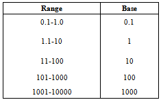
Here, the average-based length method (Huarng, 2001b) can be applied to determine the appropriate . Length of intervals significantly affects forecasting results in fuzzy time series. Hence, an effective length of intervals can significantly improve the forecasting results. The distribution based is one of the method of fuzzy time series model which can be used to adjust the lengths of intervals determined during the early stages of forecasting when the fuzzy relationship are formulated.

The distribution length of interval l is computed by the following steps:

1. Calculate all the absolute differences between the values and as the first differences, and then compute the average of the first differences.

2. Take one-half of the average as the length.

3. Find the located range of the length and determine the base.

4. According to the assigned base, round the length as the appropriate .

Table 2. Base mapping table

Step 4: Define fuzzy numbers:

The number of intervals (fuzzy numbers), m, is computed by

(3)

Thus, there are m intervals and m fuzzy numbers, which are and respectively. Assume that the m intervals are, , , . . . , , , and . The fuzzy numbers can be defined as follows.

,

,

.

.

.

,

Step 5: Fuzzify the historical data:

If the value of is located in the range of , then it belongs to fuzzy number . All must be classified into the corresponding fuzzy numbers.

Step 6: Generate the fuzzy logical relationships:

For all fuzzified data, derive the fuzzy logical relationships based on definition 3:

The fuzzy logical relationship is like , which denotes that “if the value of time is , then that of time t is ”.

Step 7: Establish the fuzzy logical relationship groups:

The derived fuzzy logical relationships can be arranged into fuzzy logical relationships groups based on the same fuzzy numbers on the left hand sides of the fuzzy logical relationships. The fuzzy logical relationship groups are like the following

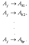Step 8: Calculate the forecasted outputs:

The forecasted value at time t, , is determined by the following three heuristic rules. Assume the fuzzy number of at time is .

Rule 1:

If the fuzzy logical relationship group of is empty; , then the value of is , which is .

Rule 2:

If the fuzzy logical relationship group of is one to one; , then the value of is , which is .

Rule 3:

If the fuzzy logical relationship group of is one to many , , . . . , , and then the value of is calculated as follows.

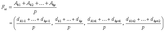where,

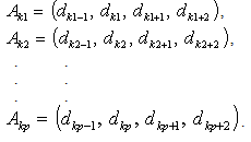
2.3. Performance of Models

The following measures of goodness of fit have been used to judge the adequacy of the model developed.

Root Mean Square Error (RMSE) =

Mean Absolute Error (MAE) = , and

Mean Square Error (MSE) =

Average Forecasting Error Rate (AFER) =

where n and p are number of observations and number of parameters, respectively in the model. The lower the values of these statistics, the better were the fitted model.

As pointed out by Kvalseth[12], before taking any final decision about the appropriateness of the fitted model, it is paramount importance to investigate the basic assumptions regarding the error term, viz., randomness and normality.

Randomness assumption of the residuals needs to be tested before taking any final decision about the adequacy of the model developed. To carry out the above analysis “Run test” procedure is developed in the literature

2.4. Test for the Randomness of the Residuals

To test the randomness of the residuals the following hypothesis was tested

H₀ : the set of residual was random Vs H₁: the set of residual was not random

Let N1 be the number of residuals of one type and N2 be the number of residuals of other type. r is the number of runs (sequence of symbols of one kind separated by symbols of another kind). If both N1 and N2 are less than or equal to 20, then table in the Appendix gives the critical values of r under H₀ for α = 0.05. If the observed value of r falls between critical values, H₀ cannot be reject. If the observed value of r is equal to or more extreme than one of the critical values, H₀ should be rejected (Sidney Siegel and John Castellan N, Jr.[21]).

2.5. Test for Normality of the Residuals

The Shapiro – Wilk[20] statistic was used to test whether the residuals are normally distributed or not. The test is based on n residuals. These were arranged in non – decreasing sequence and is designated by e₍₁₎, e₍₂₎, e_(3),…,e_(n). The following hypothesis was to be tested.

H₀: The residuals are normally distributed Vs H₁: These are not normally distributed.

The required test statistic W is defined as where 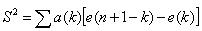. The parameter K takes the values

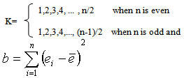The values of coefficients “a(k)” for different values of n and k are given in table 5 (Shapiro – Wilk[20]). H₀ was accepted if the value of W is very close to one.

3. Results and Discussion

Different non-linear models have been employed to study trends in the paddy crop production data presented in Appendix. The characteristic fitted non-linear models are presented in table 3. Among the non-linear models, appropriate model has been selected based on highest R² values, significance of the model parameters, lowest values of RMSE and MAE values. Residuals of the selected model would be tested for randomness and normality. Further Fuzzy time series model was employed and finally appropriate model was selected based on lowest values of MSE, RMSE, MAE and AFER which is desirable. The findings are discussed in sequence, as follows.

3.1. Non-Linear Models Fitting for Paddy Crop Production Data

Among the non-linear model fitted to the production of paddy crop, the result presented in table 3 reveals that, the maximum adjusted R² of 63 % was observed in case of Rational function model with minimum values of MSE (692484.40), RMSE (832.16) and MAE (635.93). However the residuals due to this model were not found to be normally distributed since the S-W test statistic value was significant. Hence the Rational functional model was not found to be suitable model to fit the trends in production of the paddy crop.

But the Sinusoidal model had next highest adjusted R² of 61 % with comparatively lower values of MSE (728757.80), RMSE (853.68) and MAE (651.04). Also all the estimated parameter values have been found within 95% confidence interval indicating that parameter values were significant (table 3). The model able to explain 62% of variation presents in the paddy production data. Hence among the Non-linear model fitted the following Sinusoidal model was found suitable to fit the trends in Paddy crop production. The observed and predicted values are given in table 4. and depicted in Figure 1.

Y = 4560.98^*+1528.15^*cos(0.0695^*x-3.1527^*) (R²=61%)

Similar type of trend was also reported by Rajarathinam and Vinoth[17] for the wheat crop grown during the period from 1950-51 to 2009-10 in India.

Rajarathinam and Parmar[15] reported that none of the linear and non-linear models have been found suitable to fit the trends on castor crop grown during the period from 1949-50 to 2007-08 in middle Gujarat region, India.

Rajarathinam et al.,[16] used the Rational function model to fit the trends in production of tobacco crop grown during the period 1949-50 to 2007-08 in Anand region, Gujarat State, India.

From the above discussion it can be concluded that appropriateness of the model is influenced by the type of crop as well as location.

Table 3. Characteristics of fitted Non-Linear models for the paddy crop production

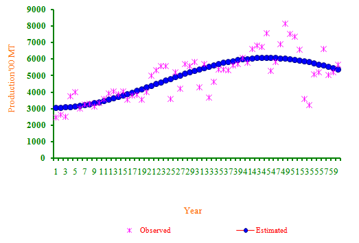Figure 1. Trends in paddy crop production based on Sinusoidal Non-linear Model

Table 4. Observed and Estimated Values for paddy productions based on Sinusoidal Non-linear Model

3.2. Fuzzy Time Series Modeling

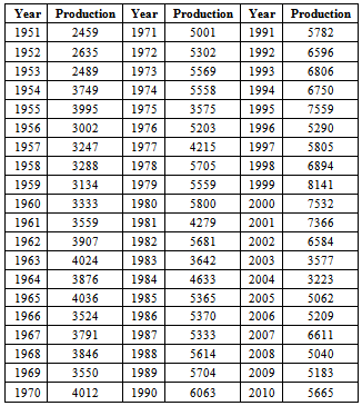
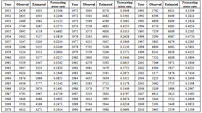
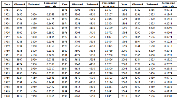
Fuzzy time series modeling have been employed to the paddy production data and the results are being discussed as follows.

The following steps have been carried out to estimate the paddy production.

Step 1: Algorithm of this method is being implemented on the Paddy crop production grown in the state of the Tamil Nadu, India during the period 1951 to 2010.

Step 2: Appendix shows that the maximum and the minimum number of the paddy productions are 8141 and 2459, respectively. For easy computation, let and . The universe of discourse U is defined as follows:

Step 3: The appropriate length of interval can be computed as follows:

1. Based on table 2, we can calculate the average of the first differences, which is 667.

2. Take one-half of 667 as the length, which is 333.5.

3. Since the length 333.5 is located at the range[101, 1000] in table 2, the base is assigned to be 100.

4. According to the base 100, the length 333.5 is rounded off to 300, which is the appropriate length of interval .

Step 4: Use Eq. 3 to calculate the number of intervals (fuzzy numbers) as follows:

.

Thus, there are 22 intervals, which are

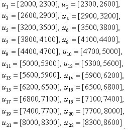The fuzzy numbers can be defined by

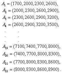Step 5: Fuzzify the productions. For example, the paddy production in year 1951 is 2459, which is located at the range of . Thus, the corresponding fuzzy number of year 1951 is assigned as .

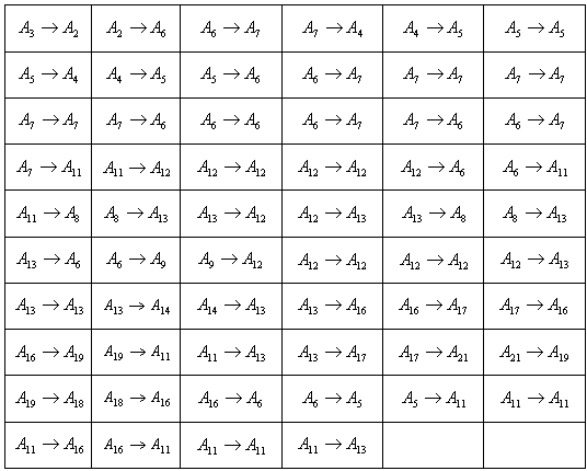
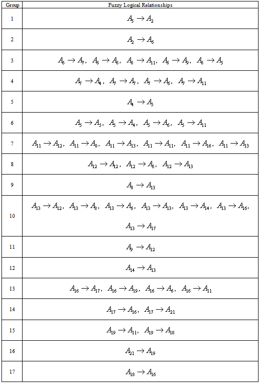
table 5 lists the corresponding fuzzy number for the paddy production of each year.

Step 6: According to table 5, we can derive the fuzzy logical relationships as shown in table 6. Notice that the repeated relationships are counted only once.

Step 7: Based on the same fuzzy numbers on the left hand side of the fuzzy logical relationships in table 6, 17 fuzzy logical relationship groups are generated as shown in table 7.

Step 8: According to tables 5 and 7, we can calculate the forecasted paddy productions. For instance, the forecasted paddy productions of years 1952 and 1954 can be illustrated below:

Forecasting 1952: The fuzzified paddy production of year 1951 in table 5 is , and from table 7, we can find that there is one fuzzy logical relationships in group 1. .

According to Rule 2, the forecasted paddy productions of year 1952 is. Thus,

Forecasting 1953: According to table 7, we can find that there is one fuzzy logical relationships in group 1. . The forecasted paddy production of year 1953 is. Thus,

Forecasting 1954: Because the fuzzified paddy production of 1954 in table 5 is , and from table 7, we can find that there are five logical relationships in group 3.

.

According to Rule 3, the forecasted paddy production of year 1954 is computed as follows:

.

Table 5. Corresponding fuzzy numbers of the paddy productions

Similarly, we can calculate the forecasted paddy production for the remaining years. Table 8 shows that the paddy productions during 1951 to 2010.

The observed and estimated paddy production data based on fuzzy time series modeling is given in the table 8 and depicted in the Fig.2.

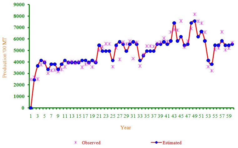Figure 2. Trends in paddy production based on Fuzzy time series modeling

Table 6. Fuzzy Logical relationships of the paddy productions

Table 7. Fuzzy logical relationship groups

Table 8. Observed and Estimated Values for paddy productions based on Fuzzy Time series Model

It is clear from the table 9 that the values of RMSE, MAE, MSE and AFER obtained using Fuzzy time series models were found to be much lower than that obtained through the non-linear model, thereby indicating the superiority of Fuzzy time series over the parametric approach. Hence Fuzzy time series model have been justified to fit the trends in production of paddy crop. The graph of the fitted trend for production of paddy crop using Fuzzy time series model is depicted in Fig.2.

Table 9. Characteristics of Model Performance parameters

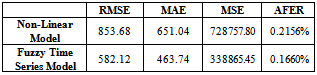
4. Conclusions

After the through analytical implementation of different non-linear and fuzzy time models over the paddy production data it can be finally concluded that, the Fuzzy time series method was justified to be a suitable method to fit the trends in paddy crop production. Fuzzy time method can be used as a more suitable one since it proved to be dynamic and versatile enough to be considered for the statistical interpretation for the trends in paddy crop production for the years to come.

Appendix

Paddy production of the Tamil Nadu data during the period 1951 to 2010