Abas Lafta1, Suaad Khalaf Salman2, Nathier Ibrahim3
1Dean, College of Administration & Economic, Wasit University, Iraq
2Department of Mathematics, College of Education for pure Sciences, Karbala University, Iraq
3Economics and Mathematics, Design, Business Administration, Al-Nahrain University, Iraq
Correspondence to: Nathier Ibrahim, Economics and Mathematics, Design, Business Administration, Al-Nahrain University, Iraq.
| Email: |  |
Copyright © 2012 Scientific & Academic Publishing. All Rights Reserved.
Abstract
AbstractThis paper deals with a new probability distribution obtained from mixing Pareto (two parameters  ) with Wiebull (two Parameters
  ), using mixing proportion
  . The researcher construct the probability density function, and cumulative distribution function, reliability, hazard functions, moments are obtained the parameters which estimated by moment method (MOM) and maximum likelihood method (MLE) using simulation procedure taking different sample size
  and replicate
  for each experiment.The comparison has been done through mean squares error (MSE).
Keywords:
KeywordsMixture distribution ( ), Pareto and Weibull, Moment Estimators, Maximum Likelihood Estimators, Mean Squares Error, Reliability
Cite this paper: Abas Lafta, Suaad Khalaf Salman, Nathier Ibrahim, Estimating Parameters and Reliability for a New Mixture Distribution  , American Journal of Mathematics and Statistics, Vol. 3 No. 4, 2013, pp. 204-212. doi: 10.5923/j.ajms.20130304.04.
1. Introduction [3][6][7]
A mixture distribution is a compounding of statistical distributions, which arise when sampling frominhomogeneous populations (or mixed populations) with a different probability density function in each component.For example the distribution of times to failure in a mixture of good and defective items, and the distribution of some diagnostic measure in a mixed population of patients, some of whom have a given disease and some of them do not have. The application of finite mixture models arise in economics, medicine, psychology, agriculture, life testing and reliability. In many applications, the available data can be considered as data coming from a mixture population of two or more distributions.This idea enables us to mix statistical distribution to get a new distribution carrying the properties of its components. The distribution constructed here is denoted by ( ), mixture of two parameters Pareto and two parameters Weibull.
2. Distribution
Here the  distribution is a mixture of some distributions with Weibull distribution, like exponential Weibull, Pareto Weibull, ErlangWeibull, Gamma Weibull. Now we explain
  distribution which is a mixture of Pareto distribution with Weibull distribution and we shall denoted it by
  The statistical properties of (
 ) are explained, then we want to estimate its parameters;a. The probability density function
  is;
is;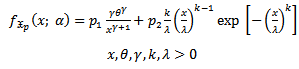 | (1) |
( ) parameters of
 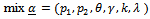 vector of parameters.b. The cumulative distribution function
  is;
is;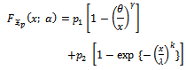 | (2) |
Also this function can be drawn for various values of parameters.The reliability function of ( ) distribution denoted by;
 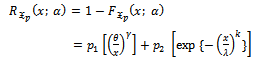 | (3) |
c. The hazard function of ( ) is;
) is;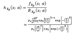 | (4) |
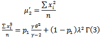
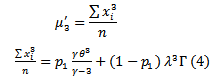
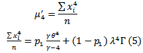
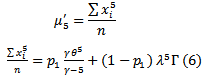
d. The  moment about origin of (
 ) distribution which can be used in estimation method are defined as;
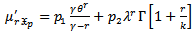 | (5) |
Where;  existing only for
  The mean and variance of (
 ) distribution can be obtained from (5), where;
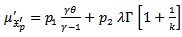 | (6) |
While the variance of ( ) is;
) is;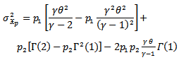 | (7) |
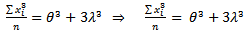
To estimate parameters by moments we must find, 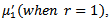 and another four moments.
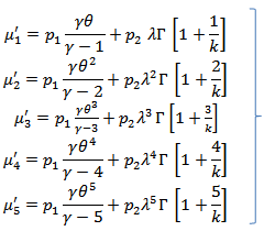 | (8) |
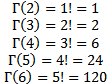
When  is integer
  for example then solving these equations yield moment estimator.
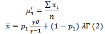 | (9) |
 | (10) |
 | (11) |
 | (12) |
 | (13) |
 Here we assumed
  if we assume
  the parameters reduced to
  since
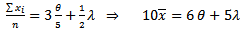
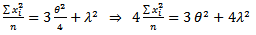
since  so we construct three equations for moment methods;
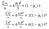 Assume
 | (14) |
 | (15) |
 | (16) |
From equation (14), find  If
If 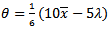 , substitute in (15);
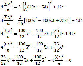 By using fixed point method where
  get;
get;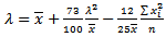 | (17) |
Using simple program, the moment estimator of  is obtained, therefore;
 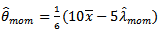 | (18) |
From  we can estimate
  by moment estimator from solving;
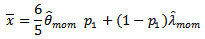 And from equation (8) since;
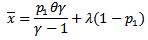 Use
Use  to obtain
3. Maximum Likelihood Method[5]
To apply the ML for the mixture distribution  from two subpopulation (
 ), where (
 ) is Pareto population and
  is Weibull population and we assume
  is mixing proportion parameters, where
  . Let
. Let  is the time failure for random sample
  taken from mixed distribution
  if we can determine the units of each sub population
  then choosing the random variable
  which is the time through it the failure time of
  units can be determined before
 such that;
 Therefore the sample units are of type (time censored sampling Type 1) and the conditional function for time failure from
  for units that failed before time
  is;
is;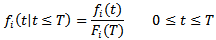 The probability that
  unit from
  failed before
  unit from
  failed before
  also, and
  is remained until time
  , is;
, is;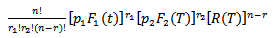 | (9) |
Then the likelihood function for sample is;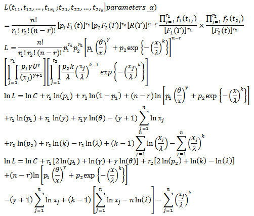 The parameters here are
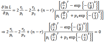 Therefore;
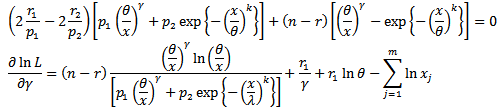
4. Simulation Procedure
We have;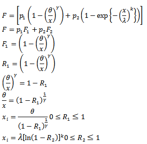 To find the estimators of (MOM & MLE), we perform simulation experiments using Monte Carlo assuming that;
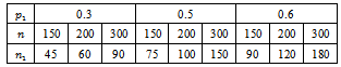 Chosen values of parameters are;
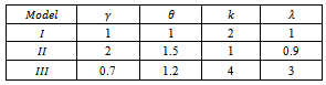 Also chosen values for predetermined censoring time (T).
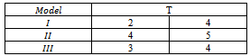 Also the total number of time intervals
  are;
are;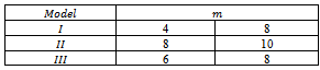 The results for estimators of parameters are explained in the following tables;
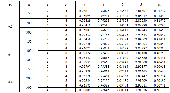
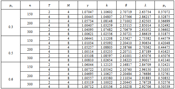
Table (1). Values of (MLE) estimatorsfor parameters of
 distribution for model I, (L=1000) distribution for model I, (L=1000)
 |
| |
|
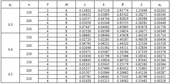
Table (2). Values of (MOM) estimatorsfor parameters of
 distribution for model I, (L=1000) distribution for model I, (L=1000)
 |
| |
|
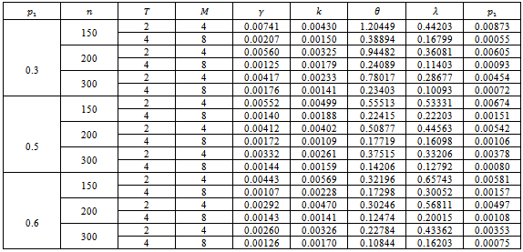
Table (3). Values of MSE for MLE estimators of
 distribution for model I, (L=1000) distribution for model I, (L=1000)
 |
| |
|
Table (4). Values of MSE for MOMestimators of
 distribution for model I, (L=1000) distribution for model I, (L=1000)
 |
| |
|
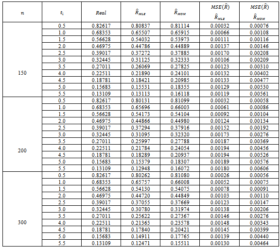
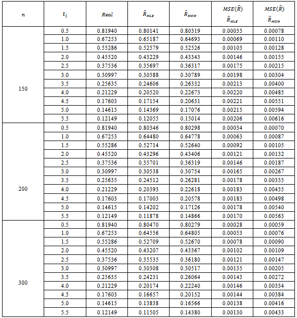
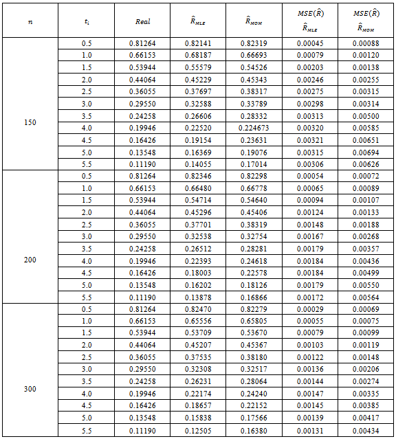
Table (5). Values of reliability function estimator by MLE , MOM & MSE
 for model I for model I

 |
| |
|
Table (6). Values of reliability function estimator by MLE, MOM & MSE
 for model I for model I

 |
| |
|
Table (7). Values of reliability function estimator by MLE , MOM & MSE
 for model I for model I

 |
| |
|
5. Conclusions
From simulation experiments, the results indicate that:1-The maximum likelihood estimator for reliability function is better than the moment estimator of reliability function.2- When  the values of estimator
  by MLE and MOM, and also of MSE
  , are convergent inspite of increasing sample size.3- The estimator of
  by MLE, and MOM approximated from real values of R by increasing the size of sample
  from
from  .4- The values of real function (R) are increasing with (T).5- The values of mean square errors for estimated parameters are decreased when (T) increasing, this is due to decreasing to failure for units drawn from each sub – population.
References
| [1] | Demidenko, E., 2004. Mixed Models: Theory and applications.Wiley, New Jersey. |
| [2] | Forbes C. E. M. N. & P.B., (2011), "Statistical Distribution" Canda. |
| [3] | Hanaa H. Abu-Zinadah, (2010), "A Study on Mixture of Exponentiated Pareto and Exponential Distributions" Journal of Applied Sciences Research, 6(4): 358-376, 2010 |
| [4] | Jiang, R., Murthy, D.N.P., Ji, P., 2001. Models involving two InverseWeibulldistributions.Reliab.Eng. Sys.Safet. 73 (1), 73–81. |
| [5] | K. Krishnamoorthy, Y. Lin, Y. P. Xia, (2009), " Confidence limits and prediction limits for a Weibull distribution based on the generalized variable approach"[Quick Edit] [CiTO] Journal of Statistical Planning and Inference, Vol. 139, No. 8. (Aug 2009), pp. 2675-2684, doi:10.1016/j.jspi.2008.12.010. |
| [6] | Maclachlan, G., Peel, D., 2000. Finite Mixture Models.Wiley, NewYork. |
| [7] | Mahir, and Ali, (2009), " Comparing two Weibull distributions using a mixing parameter", European Journal of Scientific Research. Vol.31, No.2, pp.296 – 305. |
| [8] | McCulloch, C.E. and S.R. Searle, 2001. Generalized, Linear, and Mixed Models. Wiley, New York. |
| [9] | Michel J. M., M. K. and R. P.(2004), " Bayesian Modeling and Inference on Mixtures of Distributions. |
| [10] | Mosler, K. and Scheicher, C. (2004), "Homogeneity testing in a Weibull mixture model", wiso.fak / wisostatsem / publications / Htiawmm / www.uni.koeln de / wmlx.pdf. |
| [11] | Mubarak, M. (2011), " Mixture if two Frechet Distributions: Properties and estimation", International Journal of Engineering Science and Technology (IJEST), Vol.3, No. 5, 4067 – 4073. |
| [12] | Nagode M, Fajdiga M (2006). “An Alternative Perspective on the Mixture Estimation Problem.”Reliability Engineering & System Safety, 91, 388–397. |
| [13] | Seidel,W., Mosler, K., Alker, M., 2000. A cautionary note on likelihood ratio tests in mixture models. Ann. Inst. Statist.Math. 52, 481–487. |
| [14] | Sultan, K. S., Ismail, M. A. Al-Moisheer, A. S. (2007), " Mixture of two inverse WeibullDistributions:Properties and estimation", Computational Statistics and Data Analysis, 51, 5377 – 5387. |
| [15] | Touw AE (2009). “Bayesian Estimation of MixedWeibullDistributions.”ReliabilityEngi- neering& System Safety, 94, 463–473. |
| [16] | Tsionas, E. G. (2002), "Bayesian analysis of finite mixtures of Weibull distributions", Commu. Stat. theory method, Vol. 31, No. 1, pp. 37 – 48. |
| [17] | Z. Yang, M. Xie, A. C. M. Wong, (2007), " A unified confidence interval for reliability-related quantities of two - parameter Weibull distribution" [Quick Edit] [CiTO]Journal of Statistical Computation and Simulation, Vol. 77, No. 5, pp. 365-378, doi:10.1080/00949650701227452. |
 Abstract
 Reference
 Full-Text PDF
 Full-text HTML