Bonyah Ebenezer1, Emmanuel Harris2, Farai Nyabadza3
1Department of Mathematics and Statistics, Kumasi Polytechnic Institute, Kumasi, Ghana
2Department of Mathematics Kwame Nkrumah University of Science and Technology, Kumasi, Ghana
3Department of Mathematical Science, University of Stellenbosch, South Africa
Correspondence to: Bonyah Ebenezer, Department of Mathematics and Statistics, Kumasi Polytechnic Institute, Kumasi, Ghana.
| Email: |  |
Copyright © 2012 Scientific & Academic Publishing. All Rights Reserved.
Abstract
Buruli ulcer is a neglected tropical skin disease caused by Mycobacterium ulcerans (MU) and is highly endemic in West Africa. The disease infects the skin and subcutaneous tissues, resulting in indolent ulcers, with lesions appearing mainly in the limbs. If left untreated BU may lead to extensive soft tissue destruction, with inflammation extending to deep fascia if patient do not report early for treatment. The paper applied Autoregressive Integrated Moving Average (ARIMA) time series model to examine the dynamics of Buruli ulcer dieases and also to make monthly three years forecasts. Monthly Buruli ulcer case data from 2005 to 2011 was obtained from Ashanti regional Disease Control Unit, Kumasi and analysed employing ARIMA. The results showed that in general, the trend of Buruli ulcer disease peaked during 2006.The analysis revealed that ARIMA (1, 1, 1) was the best model for forecasting Buruli ulcer disease. The forecast showed that the disease will continue to spread at faster rate then the present situation unless sometime is done now.
Keywords:
Buruli ulcer, Autoregressive (AR), Moving Average (MA) and ARIMA
Cite this paper: Bonyah Ebenezer, Emmanuel Harris, Farai Nyabadza, Forecasting Buruli ulcer Disease in Ashanti Region of Ghana Using Box-Jenkins Approach, American Journal of Mathematics and Statistics, Vol. 3 No. 3, 2013, pp. 166-177. doi: 10.5923/j.ajms.20130303.10.
1. Introduction
Mycobacterium ulcerans (MU), a pathogenic bacterium that causes dermal ulcers known as “Buruli ulcer” (BU), is fast becoming a debilitating affliction in many countries worldwide. Buruli ulcer has emerged in recent times as an important cause of human morbidity around the world, partly due to environmental changes. The incidence of BU is not limited solely to tropical environments but it has also well been documented in both the subtropical and temperate regions[5]. Buruli ulcer has been reported in over 30 countries mainly with tropical and subtropical climates but it may also occur in some countries where it has not yet been recognized such Burkina Faso and Guinea[1]. Prevalence rates in endemic districts in Ghana are reported to be up to 150 per 100,000 persons[8]. Ghana is currently the most endemic Buruli ulcer nation after La Cote d’Ivoire. WHO[12] reported that out 50,076 cases of Buruli ulcer recorded around the world, Africa tops the list of the most-affected region with Cote d’Ivoire leading the rate with a population of 2,697 patients and Ghana follows the trend with 1,048 recorded cases. In addition, Ashanti region has the highest forest-resource in Ghana also has the highest number of reported cases of the disease[8].MU is the third most mycobacterial infection after Tuberculosis (TB) and leprosy, and is the most poorly understood of these three diseases[2]. The disease infects the skin and subcutaneous tissues, resulting in indolent ulcers, with lesions appearing mainly in the limbs. If left untreated BU may lead to extensive soft tissue destruction, with inflammation extending to deep fascia if patient do not report early for treatment[3] Consequently, complications may include contractual deformities, long term disability such as restriction of joint movement as well as the obvious cosmetic problem. Early diagnosis and treatment are vital in preventing such disabilities. In Ghana for example, the disease seems to affect mostly impoverished inhabitants in remote and rural areas; children are the most vulnerable, accounting for about 70% of the cases[4]. The incidence of infection has increased dramatically over the past decade, even after considering improved reporting rates, largely as a consequence of environmental changes[8]. The large number of cases and the complications currently associated with the disease as well as the its long-term socio-economic impact could have a substantial effect on the rural economy. The long-term socioeconomic impact of Buruli ulcer on the rural economy could be substantial. In Ghana, the average cost of treatment per patient is estimated to be US $783[4]. Inadequate knowledge of the diseases has more often resulted in significant delays in the diagnosis and treatment of these cases. Time series has been employed extensively in the assessment of health science[9]. In the area of health science research, there is usually an obvious time lag between response and explanatory variable[10]. In this regard, some studies deal with this by examining models with simultaneous multiple lags of the explanatory variable[11].Forecasting Buruli ulcer incidence in Ashanti region by applying time series models would provide vital information for the region. This study aimed at developing time series models to forecast the monthly Buruli ulcer incidence in Ashanti region of Ghana based on reported incidence available from 2005-2011. This forecast offers the potential for improved contingency planning of public health intervention in Ashanti region.
2. Materials Method
Ashanti region is centrally positioned in the middle belt of Ghana. It lies between longitudes 0.150W and 2.250W and latitude 5.500N and 7.460N. This region is divided into 27 districts. Kumasi metropolis only account for almost one-third of the entire region population[7]. The city is located in the south-central part of the country, about 250km by road northwest of Accra, the capital city of Ghana.Kumasi lies at the intersection of latitude 6.040N and longitude 1.280W, covering an area of about 220 km2. This metropolis is the most populous district in the region. It has a population nearly 2 million[7] which account for more than one-third of the entire population in the region. Kumasi has attracted such a large population because of it is most commercialized city in the region and also it is centrally located as far as the entire country is concern. The city has so many satellite market but traders prefer to sell in the night where the city largest lorry park is located. People ability to eat and rest is now the thing of the past creating many cardiac health related issues in the metropolisData SourcesIn order to achieve the stated objective, we collected data on hypertension disease from regional Disease Control Units (DCU) in the Kumasi metropolis recorded monthly basis from 2005 to 2011. The data were model employing Autoregressive Integrated Moving Average (ARIMA) stochastic model made known by Box-Jenkins[6].
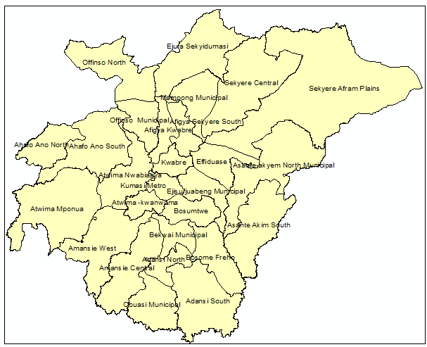 | Figure 1. Map of Ashanti region of Ghana indicating District names |
A given ARIMA  is expressed as a combination of Autoregressive
  which indicates that there is a relationship between present and past values, a random value and a Moving Average model which indicates that the present value has an association with the past residuals. The ARIMA process can be explained as :
 where
where  =Buruli ulcer cases
 = the mean of
  ,
,

 =The
=The  autoregressive parameter
 = The
= The  moving average parameter
 and
and  represent the autoregressive, moving average and differenced order parameter of the process respectively.
  and Q represent the difference backward shift operators respectively. We examine the three steps that involves in the estimation of the model. They are identification, estimation of parameters and diagnostic checking.Identification step: deal with use of the techniques to obtain the values of
  and
and  . The values are computed using Autocorrelation function (AFC) and Partial Autocorrelation function (PACF). In any given ARIMA
  process, the theoretical PACF has non-zero partial autocorrelation at lags
  and has zero partial autocorrelation at lags
  and zero autocorrelation at all lags. We accept the non-zero lags of the sample PACF and ACF as the
  and
and  parameters. The non stationary series data is passed through differencing to make the series stationary. The order of
  is determined by the number of time a data is differenced. We express stationary data
  and ARMA
  is put as
  .Estimation of parameters: involve the tentative models selected parameters.Diagnostic checking: the estimated model has to pass some test to ensure that it adequate represents the series. The diagnostic check are done on the residuals to see if they are randomly and normally distributed. In this regards, the Anderson-Darling test for normality was applied. The ACF and PACF plot of the residuals were looked at to check if the residuals are white noise. The correlation matrix of the estimated parameters was tested to check if any of the parameters are correlated so that such variables can be done away with. The Ljung-Box Q statistics was used to check the overall adequacy of the model. The test statistics is expressed as :
 where
where  = the residuals autocorrelation at lag
 = the number of residuals
 = the number of time lags included in the test.In any instance, when the
  -value associated with the Q is large the model is said to be adequate, otherwise the whole estimation process has to be begin again so that the most adequate model is
3. Results and Discussions
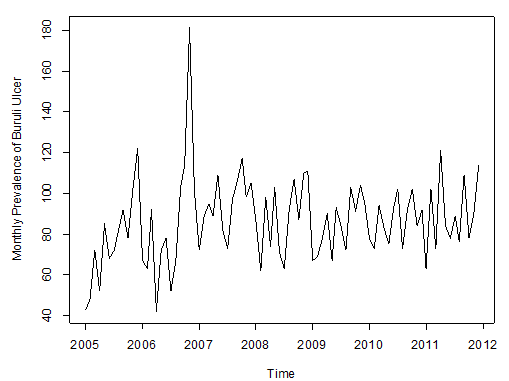 | Figure 2. Observed Prevalence of Buruli ulcer cases from JAN, 2005 to DEC, 2001 |
Figure 2 above shows the pattern of monthly Buruli ulcer cases recorded in the Ashanti Region of Ghana between January, 2005 and December, 2011.We observe random fluctuations with maximum peak in 2006 (i.e. during November), which recorded a total of 181 ulcer cases. The minimum recorded figure also occurred in that year in the month of April. Also, the pattern of the monthly data looks trend stationary from 2007 to 2011.Furthermore, the data is then decomposed to make more evident the existence/ non-existence of the various components of the series. This is shown in Figure 2 below. | Figure 3. Decomposition of the Buruli ulcer series |
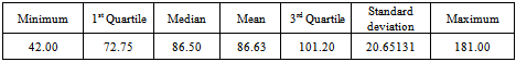
After decomposition, it is observed clearly that the data exhibits no systematic linear trend but the existence of seasonality is suggested. This is because the pattern displayed in Figure 3 could be as a result of the irregular component in the time series.Table 1. Summary Statistics of Buruli Ulcer data
 |
| |
|
From table 1, we observed that the minimum number of Buruli ulcer cases recorded is 42, which occurred in April, 2006.The maximum number recorded is 181 which also occurred in November, 2006.The average number of Buruli ulcer cases is approximately equal to the median number of Buruli ulcer cases recorded throughout the period. This may indicate some symmetric behaviour of the Buruli ulcer distribution. In order to achieve stationarity, the observed data looks trend non-stationary for certain period, we differenced it to remove that little element of trend. After the first order differencing, the Buruli ulcer data series now assumes the pattern below;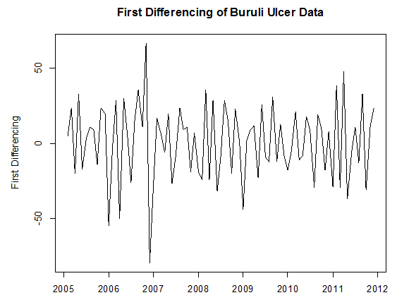 | Figure 4. Pattern of First Differenced Buruli ulcer Data |
From Figure 4 above, it can be seen that the differenced series looks stationary for all periods, as the observations seem to beat about a mean of zero. Testing Stationarity of Differenced Data, we performed theKwiatkowski-Phillips-Schmidt-Shin (KPSS) test on the difference data series. The results obtained for the test were KPSS Level = 0.0362, Truncation lag parameter = 2 and p-value = 0.1. Therefore, at an α (alpha) 5% level of significance, we fail to reject the Null hypothesis that the difference series is trend or level stationary since the p-value (0.1) > 0.05, and hence conclude that the series is indeed trend stationary.We examined seasonlaity by testing that if there is significant seasonality, the autocorrelation plot should show significant spikes at lags equal to the period of the series. For example, for monthly data, if there is a seasonality effect, we would expect to see significant peaks at lag 12, 24, 36, and so on (although the intensity may decrease the further out we go).From Figure 5 below, it can be seen from the sample ACF that lags 12 and 24 lie within the significant bounds, hence showing no significant peaks. The sample ACF therefore shows no obvious pattern of seasonality. Also, since the data series was differenced once to attain stationarity, we can therefore conclude that our data is non-seasonal. This is because for non-seasonal data, at most a first order differencing is usually sufficient to attain apparent stationarity.
4. Model Identification
In order to select the appropriate model and also make more accurate forecasts, we fitted several feasible ARIMA models to the observed data by making reference to the Sample ACF and Sample PACF (in Figure 4 above) of the difference data. Since the data was difference to attain stationarity (as shown by the KPSS Test), the fitted ARIMA models would be of order (p, d=1, q).From the correlogram in Figure 5, the sample ACF has only lag 1 and lag 18 exceeding the significant bound, with most lags dying down. Lag 18 is however ignored, because this may be due to chance. After all, the probability of a spike being significant by chance is about one in thirty.Also the partial correlogram shows that the partial autocorrelations at lags 1 and 2 cuts the significant bounds consistently, with lag 10 also exceeding. However, lag 17 just touches the bounds. The partial autocorrelations tails off after lag 17. From the foregoing analysis, the following ARIMA (Autoregressive integrated moving average) models are therefore plausible for the data series: • ARIMA(2,1,1) • ARIMA(2,1,0) • ARIMA(1,1,1) At this point we proceed to estimate and test the parameters and as well investigate whether the residuals of the selected ARIMA models are normally distributed with mean zero and constant variance, and also whether there are no correlations between successive residuals (i.e. randomness of residuals). To check for correlations between successive residuals, we made use of a correlogram and also the Ljung-Box test to further ascertain the adequacy (randomness) of the model’s residual.Also to check whether the residuals are normally distributed with mean zero and constant variance, we made use of a normality quantile-quantile plot (q-q plot) and a histogram.If the residuals are normally distributed, the points on the normal quantile-quantile plot should approximately be linear, with residual mean as the intercept and residual standard deviation as the slope whilst the shape of the histogram shows “a bell-like” shape.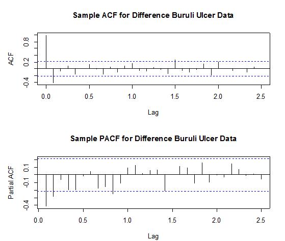 | Figure 5. Shows the Sample ACF (top) and Sample PACF (bottom) for the difference data |
• ARIMA(2,1,1)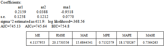
 | Figure 6. ACF of ARIMA (2, 1, 1) Residuals |
Box-Ljung test: From Figure 5 above, the ACF of residuals shows that two (2) out of the 30 lags of the sample autocorrelations cuts the significant bounds with one other lag just touching. Also, most of the other lags seem to be dying down.
 | Figure 7. Shows the Histogram (left) and Normality plot (right) for the residuals of ARIMA (2, 1, 1) |
This simply gives an indication of non-significant autocorrelation, since we would expect at most two (2) out of 30 sample autocorrelations to exceed the 95% significance bounds. Also, from the Ljung-box test above, the computed p-value (i.e. 0.1403) is greater than α (alpha) 5% level of significance.Hence from these deductions, we fail to reject the null hypothesis that the series of residuals exhibits no autocorrelation and conclude that there is insignificant evidence for non-zero autocorrelations in the residuals at all lags (i.e. the residuals are independently distributed).To check whether the residuals are normally distributed with mean zero and constant variance, we make a normality plot and a histogram of the residuals.From the plot in Figure 7, the histogram of the residuals displayed above gives an indication of a symmetric distribution, thus it shape looks “bell-like” and certainly better for the fitted model. The QQ-normal plot for the residuals also throws more light on this since most of the residuals do not deviate that much from the line of best fit and it distribution looks approximately linear. Hence, from Figure 7, it is plausible that the forecast errors are normally distributed with mean zero and constant variance. • ARMA(2,1,0)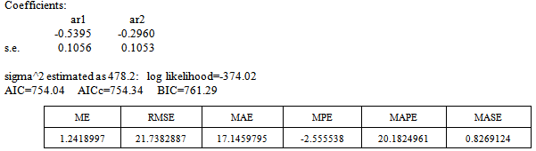
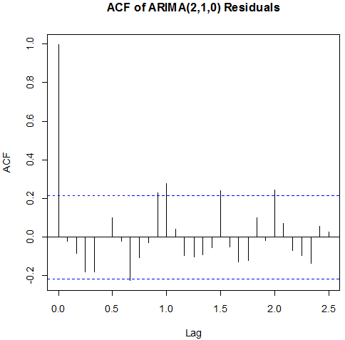 | Figure 8. ACF of ARIMA (2,1 ,0) Residuals |
Box-Ljung test: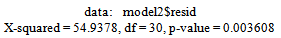 From Figure 8 above, the ACF of residuals shows that five (5) out of the 30 lags of the sample autocorrelations exceed the significant bounds, with other lags getting closer enough to the significant bound.This simply gives an indication of significant autocorrelation, since we would expect at least five (5) out of 30 sample autocorrelations to exceed the 95% significance bounds. Also, from the Ljung-box test above, the computed p-value (i.e. 0.003608) is less than α (alpha) 5% level of significance. Hence from these deductions, we reject the null hypothesis that the series of residuals exhibits no autocorrelation and conclude that there is significant evidence for non-zero autocorrelations in the residuals at all lags (i.e. the residuals are dependently distributed).To check whether the residuals are normally distributed with mean zero and constant variance, we make a normality plot and a histogram of the residuals.
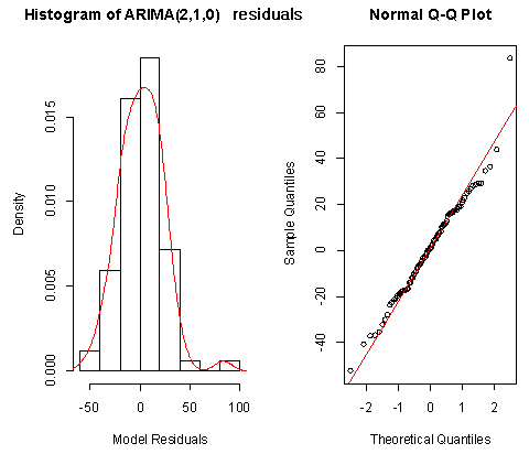 | Figure 9. Shows the Histogram (left) and Normality plot (right) for the residuals of ARIMA (2, 1, 0) |
From the plot in Figure 9, the histogram of the residuals displayed above gives an indication of a symmetric distribution, thus it shape looks “bell-like” and certainly better for the fitted model. The QQ-normal plot for the residuals also throws more light on this since most of the residuals do not deviate that much from the line of best fit and it distribution looks approximately linear. Hence, from Figure 8, it is plausible that the forecast errors are normally distributed with mean zero and constant variance.• ARMA(1,1,1)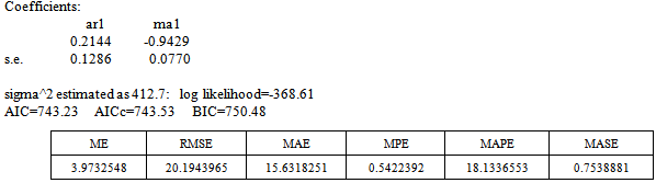
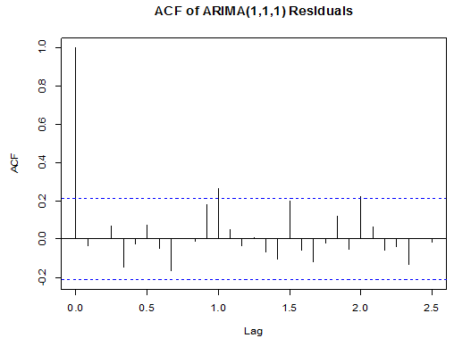 | Figure 10. ACF of ARIMA (1, 1, 1) Residuals |
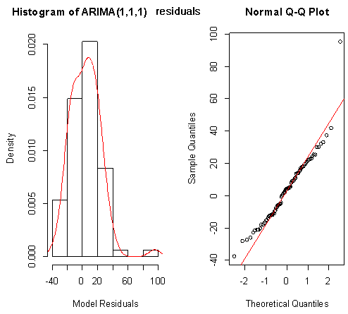 | Figure 11. Shows the Histogram (left) and Normality plot (right) for the residuals of ARIMA (1, 1, 1) |
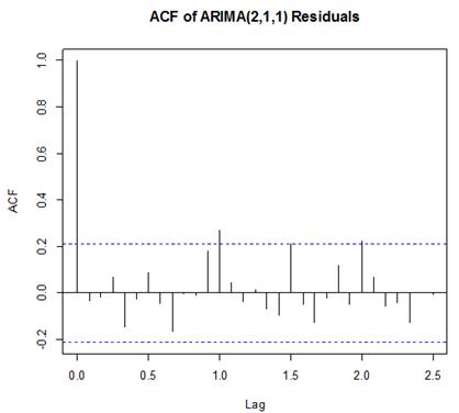
Box-Ljung test: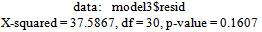 From Figure 9 above, the ACF of residuals shows that two (2) out of the 30 lags exceed the significant bounds, with just one lag getting closer enough to the bounds. Also, majority of the lags dies down.This simply gives an indication of little autocorrelation, since we would expect at most two (2) out of 30 sample autocorrelations to exceed the 95% significance bounds. Furthermore, the p-value for the Ljung-Box test computed above is 0.1607, indicating that there is little evidence for non-zero autocorrelations in the residuals for lags 1-30. Hence from these deductions, we fail to reject the null hypothesis that the series of residuals exhibits no autocorrelation and conclude that there is insignificant evidence for non-zero autocorrelations in the residuals at all lags (i.e. the residuals are independently distributed).To check whether the residuals are normally distributed with mean zero and constant variance, we make a normality plot and a histogram of the residuals.From the plot in figure 11, the histogram of the residuals shown above gives an indication of a symmetric distribution, thus it shape looks “bell-like” and certainly better for the fitted model. The QQ-normal plot for the residuals also throws more light on this since most of its residuals do not deviate that much from the line of best fit and it distribution looks approximately linear.Hence, from Figure 10, it is plausible that the forecast errors are normally distributed with mean zero and constant variance.
5. Model Selection
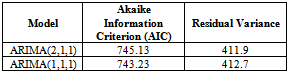
In order to select the most appropriate model for our data, we compare all competing models and select the one with the minimum AIC (Akaike Information Criterion value) and Residual Variance. From the diagnostic checks above, since ARIMA (2, 1, 0) failed to satisfy the assumption of non-autocorrelation, it fails to stand as a possible competing model.Table 2. Akaike Information Criterion for the possible Models
 |
| |
|
From table 2 above, it is clear that ARIMA (1, 1, 1) model is the best model for forecasting since its AIC and residual variance values are better than that of the other competing model. Therefore, the chosen model for the Buruli ulcer data series is of the form; This indicates that the fitted model is a linear combination of both previous Buruli Ulcer values and previous forecast error.
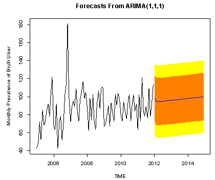 | Figure 12. The forecasted Buruli ulcer values are shown by the blue line, whilst the orange and yellow shaded areas show 80% and 95% prediction intervals respectively |
6. Forecasting
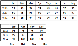
We also make forecast using the most adequate fitted model for the next three years. Below is the graph of the forecasts.The forecasted values and standard errors are given in table 3 and 4 below respectively:Table 3. Forecasted Buruli Ulcer Values Using ARIMA (1, 1, 1)
 |
| |
|
7. Conclussions
The study revealed the random fluctuations with maximum peak in 2006 which occurred during November and the minimum recorded also in that same year in the month of April. Again, the pattern of the monthly data looked trend stationary from 2007 to 2011. The best model was achieved based on various diagnosis, selection and evaluation criterion on ARIMA (1,1,1). The forecast shows an increasing tend in the spread of Buruli ulcer disease in Ashanti region of Ghana which is worrying situation for Ghana.In order to reduce the spread of the disease government should intensify the education on the disease especially in the rural areas for early reporting to health facilities. There should be alternative livelihood in most of the communities where the environment is seriously disturbed such as mining and many others.
References
| [1] | Portaels, F. 1995. Epidemiology of mycobacterial diseases. Clin. Dermatol. 13:207-222 |
| [2] | WHO,WorldReport,2005,http://www.who.int/immunization_financing/countries/gha/summary_data/en/index.html (accessed July 2009). |
| [3] | Amofah, G. K., Sagoe-Moses, C., Adjei-Acquah, C., Frimpong, E. H. 1993.Epidemiology of Buruli ulcer in Amansie West District, Ghana. Trans Roy Soc Trop Med Hyg 87, 644-645. |
| [4] | Asiedu, K., Portaels, F. 2000. Introduction. In: Asiedu, K., Scherpbier, R., Raviglione, M. (eds.). BURULI ULCER: Mycobacterium ulcerans infection, World Health Organisation, Global Buruli Ulcer Initiative, pp 5-7 |
| [5] | Portaels, F., Elsen, P., Guimaraes-Peres, A., Fonteyne, P., Meyers W.M. 1999. Insects in the transmission of Mycobacterium ulcerans infection. The Lancet 353: 986. |
| [6] | Box GEP & Jenkins GM (1976) Time Series Analysis: Forecasting and Control, Revised Edition. Holden Day, San Francisco |
| [7] | Ghana Statistical Service Population and Housing Census 2010 |
| [8] | Amofah, G., Bonsu, F., Tetteh, C., Okrah, J., Asamoa, K., Asiedu, K., Addy, J. 2002. Buruli ulcer in Ghana: results of a national case search. Emerg. Infect. Dis 8: 167-170 |
| [9] | Helfenstein, U. 1991 “The use of transfer function models, intervention analysis and related time series methods in epidemiology,” Int. J. Epidemiol, vol. 20, pp. 808-815, |
| [10] | Schwartz, J., Spix, C., Touloumi, G., Bacharova, L., Barumamdzadeh, T., Tertre,A., Pickarksi, T., Leon, A., Ponka, A., Rossi, G., M. Saez, M., J. Schouten, J. 1996 “Methodological issues in studies of air pollution and daily counts of deaths or hospital admissions,” J. Epidemiol. Community Health, vol. 50(s), pp. s3-s11, |
| [11] | J. Schwartz, J. 2000 “The distributed lag between air pollution and daily deaths,” Epidemiology, vol. 11, pp. 320-326, |
| [12] | World Health Organization (WHO) report on Buruli ulcer 2011. |
 Abstract
 Reference
 Full-Text PDF
 Full-text HTML