Abd-Elnaser S. Abd-Rabou, Ahmed M. Gad
Statistics Department, Faculty of Economics and Political Science, Cairo University, Cairo, Egypt
Correspondence to: Abd-Elnaser S. Abd-Rabou, Statistics Department, Faculty of Economics and Political Science, Cairo University, Cairo, Egypt.
| Email: |  |
Copyright © 2012 Scientific & Academic Publishing. All Rights Reserved.
Abstract
For a given data set it may be required to discover if a change has been occurred. This is can be conducted using change-point analysis. Let X1, X2, …,Xn be independent randomvariables with respective continuous distribution functions F1, F2, …, Fn such that Fi(0)=0 for all i.We consider the problem of testing the null hypothesis that F1= F2= …= Fnagainst the alternative of r-changes in the distribution functions of this sequence at unknown times 1<[nτ1]<[nτ2]< …. <[nτr]<n, where[ y] is the integer part of y. We study the asymptotic theory of change-point processes which are defined in terms of the empirical process. We propose and study new weighted non-parametric change-point test statistics for a possible change in distribution function of a data set.
Keywords:
Change Point Problem, EmpiricalProcesses, Kiefer Process, Limit Theorems, Monte Carlo Simulation
Cite this paper: Abd-Elnaser S. Abd-Rabou, Ahmed M. Gad, Non-Parametric Weighted Tests for Change in Distribution Function, American Journal of Mathematics and Statistics, Vol. 3 No. 3, 2013, pp. 157-165. doi: 10.5923/j.ajms.20130303.09.
1. Introduction
In many applications it is necessary to discover if a data set comes from a single distribution or there is a change in the distribution function. The change-point inference is an effective and powerful statistical tool for determining if and when a change in a set of data has occurred. Let X1, X2, …,Xn,be independent random variables with continuous distribution functions (DF) F1, F2, …, Fn, respectively such that Fi(0)=0for all i. We are interested in testing the null hypothesis of no change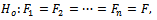 | (1) |
where F is unknown against the alternative of at most r-changes (AMRC),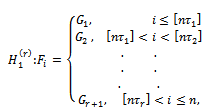 | (2) |
where  is specified, the distribution functions
  and the change-point positions
  are unknown
  Note that[τ] denotes the integer part of τ.The aim of this article is to introduce weighted non-parametric tests for distributional change in a data set. The asymptotic distributions of these test statistics are derived. These tests also can be applied to the mean change ina data set.The paper is organized as follows. In Section 2 we will consider the above multiple change-point problem in the case of at most two change-points (AMTC), i.e. r=2. In Section 3 we generalize the AMTC results to the case of
 . The proposed new change-point test statistics are presented in Section 4. Also, the asymptotic distributions of the proposed test statistics are derived in Section 4. In Section 5, we propose new test statistics for the case of at most one change point. We study the applicability of the proposed tests through a Monte Carlo study in section 6.
2. The Case of at Most Two Change Points (AMTC)
In this section we treat the case of at most 2-changes (AMTC), i.e. testing  of (1) against the alternative of (2), when r = 2.Many authors have discussed the change-point problem, testing (detection), and estimation using both Bayesian and non-Bayesian approaches. Most of the work done in the change-point analysis is concerned with the case of at most one change (AMOC). Csörgő and Horváth[1] gave avery excellent and extensive treatment and review for the related work. Forthe AMTC, recent works are done by[2,3]. They propose weighted CUSUM tests for the multiple changes in the variance of a sequence of independent random variables. By using the general form of U-statistic, they studied some CUSUM test statistics for the AMTC in variance. Hawkins[4] developed a dynamic program to test for a multiple change point in the parameters of the general exponential family using repeated maximum likelihood algorithm. His algorithm, involves the application of the at most one change-point maximum likelihood detector for every segmented group of data available.Syzsykowicz[5] studied weighted approximations for various versions of the empirical processes under the null and continuous alternatives of the AMOC. She approximated these processes by appropriate Gaussian processes.Let the smoothed two-parameter empirical process be given by
 | (3) |
Let , where
  For
For  define
 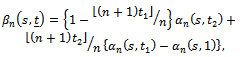 | (4) |
and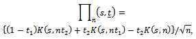 | (5) |
where  is a Kiefer process, i.e., a mean zero two-parameters Gaussian process with
  | (6) |
The following result follows from Theorem 8.2.1 of[5].Theorem 1.Assume that  of Eq. (1) holds true. Then, there exists a Kiefer process K(.,.) such that as
 where
where is as in Eq. (4) and
  is as in Eq. (5).Let
  be as in Eq. (3) and
  be as in Eq. (4). Define
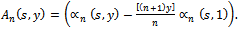 | (7) |
Note that 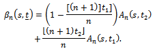 Let Q be the class of positive functions on (0,1), which are non-decreasing in a neighbourhood of zero and non-increasing in the neighbourhood of one. A function q defined on (0, 1) is called positive if
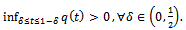 Let
Let the AMTC weighted-process,
  is defined as
 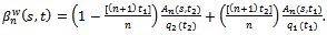 | (8) |
Let K(.,.) be a Kiefer process. Define 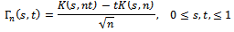 and
and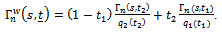 | (9) |
Note that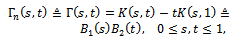 | (10) |
where  and
and  are two independent Brownian bridge.Now we give the main theorem of this section.Theorem 2.Under
  of (1), there exists a Kiefer process K(.,.) such that as
 1. if for i=1,2
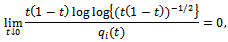 and
and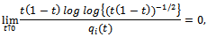 then
then 2. if for i=1,2
 then
then and
and Proof of Theorem 2 (Sketch)First we can easily notice that
  | (11) |
where the right-hand side is the two-time parameter empirical process of[5].Second if we put  in (6.1.13) of [5], we get as
 | (12) |
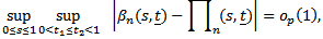
Using the definition of the processes of Eq. (8) and Eq. (9), the statements of Eq. (11), Eq. (12) and Theorem 8.3.1 of[5], we complete the proof of this theorem.Now, let  be the process defined in Eq. (8), then by Theorem (2) and the relations in Eq. (9) and Eq. (10), we have
  where
where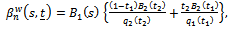 | (13) |
and  are as in Eq. (10).As in Pouliot[3], we may use the one weight function
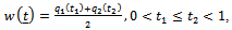 for the whole process. It is very easy to see that Theorem 2 remains true under the one-weight function
  In this case the corresponding limiting process of Eq. (13) becomes
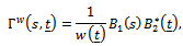 where
where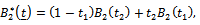 and
and  are independent Brownian bridge. It is clear that
  is a mean zero Gaussian process with covariance function
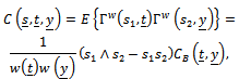 where
where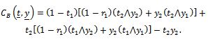
3. The Case of at Most r Change Points (AMRC)
We consider here the general case of  Following the definition of the change-point processes in (6.5) of Pouliot (2001), we define the weighted r-change point empirical process and its corresponding weighted Gaussian process as follows. Assume that
 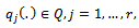 satisfy the two assumptions of part (1) of Theorem 2, we define the weighted r-time parameter empirical process
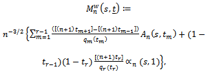 | (14) |
where 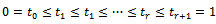 and the processes
  are defined by Eq. (3) and Eq. (7) respectively. We also define the weighted r-time parameter limiting Gaussian process as follows;
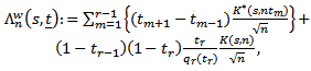 | (15) |
where K(.,.) is the Kiefer process of Eq. (6) and  Now, following the steps of the proof of Theorem 2, we can state the general weighted-sup metric approximation for the r-time parameter empirical process of Eq. (14).Theorem 3.Under the null hypothesis
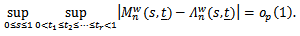
  of (1), there exists a Kiefer process K(.,.) such that with the sequence of processes
  and
and  of (14) and (15) respectively, we have as
 Under the conditions of Theorem 3, we obtain
 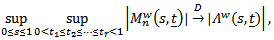 where
where  is the process in Eq. (15) when n=1.
4. The Proposed AMRC Test Statistics
To introduce our proposed multiple change-point test statistics, we need the following integrated processes. Let  be the smoothed two-parameters empirical process defined by Eq. (3).Then integrating over
  we get
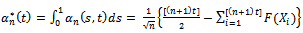 | (16) |
and define the integrated empirical process difference of Eq. (4) as;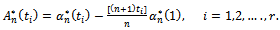 | (17) |
The generalized test statistics’ integrated processes in the case of  AMRC, and
 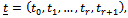 such that
 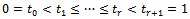 are given by
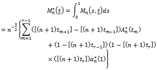 where
where  is defined by Eq. (16) and its corresponding limiting Gaussian process is
 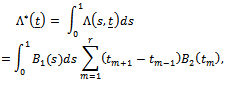 where
where  is defined by Eq. (15) and B(.) is a standard Brownian bridge defined on the same probability space.Next, we define the weighted processes
  and
and , that are needed to construct the AMRC test statistics.For
 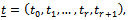 such that
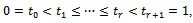 we define the following weighted processes.
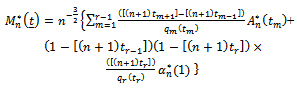 | (18) |
and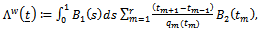 | (19) |
where  and
and  are given by Eq. (16) and Eq. (17) respectively and
 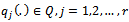 are the weight functions of Theorem 3.1 Theorem 4.Let B(.) be a Brownian bridge and assume that
  of (1) holds. Then as
 where
where  such that
  and
and  and
and  are the processes given by (18) and (19) respectively.The proof of this theorem can be deducted easily from that of Theorem 3.Corollary 1.By the continuous Mapping Theorem and for
 , we have
 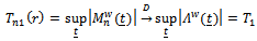 and
and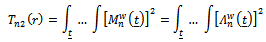 The asymptotic distribution of
  and
and  are, up to our knowledge, are unknown. For this reason we present the special case; at most one change point test statistics. Then we study the applicability of the proposed teststhrough a Monte Carlo simulation study.
5. The at Most One Change (AMOC) Test Statistics
First, we present the two-weight function test statistics for the CDF on change-point change.For  consider the following weight functions;
 | (20) |
and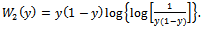 | (21) |
Let  is the empirical counterpart of the process in Eq. (16), defined by replacing the CDF, F(.), by its sample one
 . We define the test process
  by
by | (22) |
where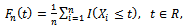 is the sample empirical distribution function. The above test process is the natural candidate in case of testing for a change in the CDF of a sequence of independent random variables.Let
  and
and  where (a, b) = (0.071033…, 0.928966…), see[3]. Now, we propose the following AMOC test statistics;
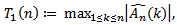 | (23) |
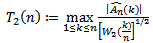 | (24) |
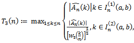 | (25) |
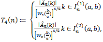 | (26) |
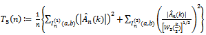 | (27) |
and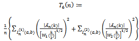 | (28) |
where  and
and  are given by Eq. (20), Eq. (21) and Eq. (22) respectively.Note that the first four test statistics are CDF change point versions analogues to Pouliot (2001). The last two
  and
and  are new proposed test statistics. The limiting distributions of the above test statistics are unknown in literature. Thus we conduct a Monte Carlo study to determine the performance of these test statistics.
6. Estimated Critical Values and Powers
The critical values of the proposed tests in (23)-(28) have been evaluated via simulation. Also, the power of the proposed tests have been estimated. These estimation tasks are conducted using three simulation studies.
6.1. Simulation 1
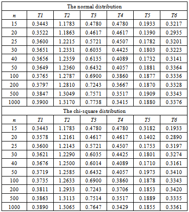
The aim of this simulation is two-folds. First, to estimate the critical values of each test at different sample sizes under different distributions.Second, to show that the critical values are stable. The upper 5% critical values for each test of the six tests given in (23)-(28) have been obtained via simulation study. A sample of each distribution has been simulated. The sample sizes are fixed at 15, 20, 25, 30, 40, 50, 100, 200, 500, and 1000. The underlying distributions are the normal distribution, the chi-square distribution, the exponential distribution and the uniform distribution. Each test value is evaluated for each sample. This process is replicated 10000 times. Then, each test values are sorted and the upper 95% percentile is obtained.The simulation results are displayed in Table 1 and Table 2. The other distributions critical values have a similar behaviour. From these results we can notice that the second test has a higher critical values followed by the third test, for all the four distributions. The fifth test has the lowest critical values across all the four distributions. The critical values of the first, fourth and sixth tests are close.Generally, the critical values of all tests starts at a higher (lower) levelfor smaller sample size; n = 15, but they converge reasonably as the sample size increase, see the table 1. This convergence appears from a sample size as large as 100.Table 1. The estimated upper 5% critical values of the normal and chi-square distributions
 |
| |
|
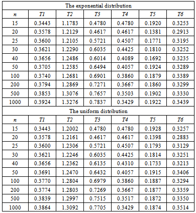
Table 2. The estimated upper 5% critical values of the exponential and uniform distributions
 |
| |
|
6.2. Simulation 2
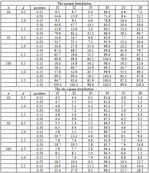
The aim of this simulation study is to estimate the power of the tests (23) - (28) assuming there is one change point in the mean. A sample of fixed size is generated fromeach distribution. The sample sizes are fixed at 20, 50, and 100 units, to cover small, moderate and large sample size. The samples are generated from the normal distribution, the chi-square distribution, the exponential distribution and the uniform distribution. The change point positions are fixed at the first tail (15%n) of the sample and in the middle (50%n) of the sample. Different change shifts have been used, namely Δ= 0.5, Δ= 1.0 and Δ= 1.5. The replications number is 10000. The percentage of times the test statistic exceeds the estimated critical values is reported for each change, test statistic, and sample size. The results are displayed in Table 3 and Table 4.The simulation results show that the estimated power of each test undereach distribution increase as the change position moves to the middle of the sample. The estimated powers of all tests increase as the change shift increases and the sample size increases.From the results we can see that the fourth test has the highest powerfollowed by the sixth test for all distributions in the different settings. The third test has the lowest power in the different setting. The estimated powers of the first and the second tests are comparable in the different settings. The powers under the uniform distribution has the highest values, whereas the lowest powers are under the chi-square distribution. This is not surprising because any change in the mean of the uniform random variable affect the distribution boundaries too. However, the chi-square distribution will change its shape very slowly with such minor location changes. Table 3. The estimated powers of the normal and chi-square distributions (change in the mean)
 |
| |
|
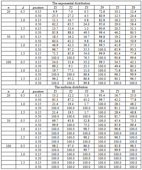
Table 4. The estimated powers of the exponential and the uniform distributions (change in the mean)
 |
| |
|
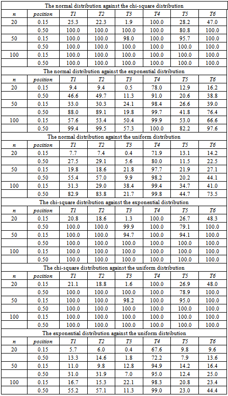
6.3. Simulation 3
The aim of this simulation is to estimate the power of the proposed testassuming that there is change point in the distribution rather than only the distribution mean. A sub-sample is simulated from a given distribution augmented by another sub-sample of another distribution. This means that there is a change in distribution. The change positions are the first 15% point of the sample and the middle of the sample. The sample sizes are fixed at n = 20, n = 50 and n= 100. Four different distributions have been used; namely the normal distribution, the chi-square distribution, the exponential distribution and the uniform distribution. The results in Table 6 show the estimated power of the tests for the normal distribution against the other three distributions (the chi-square distribution, the exponential distribution and the uniform distribution). Also, the table shows the estimated power of the tests assuming the chi-square distribution against the exponential and the uniform distribution in addition to the exponential distribution against the uniform distribution.From the results we can notice that the fourth test has the highest powerfollowed by the sixth test. Generally, the third test has the lowest estimated powers. The highestpowers are obtained for the chi-square distribution against the rest of the distributions.
7. Discussion and Conclusions
In this paper we presented new non-parametric weighted type test statisticsfor a change in the cumulative distribution function of a set of data. These proposed test statistics are based on the empirical processes. The asymptotic distributions of these test statistics are unknown and intractable to be studied theoretically.We conducted a simulation study to estimate the critical values and powersof the proposed tests in the at most one change point. Our weighted proposed tests have good performance in all settings; different distributions, different sample sizes and different change positions. The difficulty of tracing the limiting distributions of the proposed weighted test statistics encouragethe search for a simple new weighted test statistics.Table 5. The estimated powers of a distribution change
 |
| |
|
References
| [1] | Csörgő, M. and Horváth, L., 1979, Limit Theorems in Change-Point Analysis, John Wiley & Sons, New York. |
| [2] | Orasch, M. R., 1999, Multiple change-points with an application to financial modelling, Ph.D. thesis, Carleton University, Ottawa, Canada. |
| [3] | Pouliot, W. J., 2001, Non-parametric, Non-sequential change-points analysis, Ph.D. thesis, Carleton University, Ottawa, Canada. |
| [4] | Hawkins, D. M., 2001, Fitting multiple change-point models to data, Computational Statistics & Data Analysis, 37, 323-341. |
| [5] | Syzsykowicz, B., 1992, Weak convergence of stochastic processes in weighted metrics and their applications to contiguous change-points analysis, Ph.D. thesis, Carleton University, Ottawa, Canada. |
| [6] | Aly, E.-E., Abd-Rabou, A. S. and Al-Kandari, N. M., 2003, Tests for multiplechange points under ordered alternatives, Metrika, 57, 209-221. |
 Abstract
 Reference
 Full-Text PDF
 Full-text HTML