1. Introduction

A number of power consumption forecasting models have been proposed in the past using many theoretical methods including growth curve[19,3,24& 10], in their work titled “A Stochastic Bass Innovation Diffusion Model for Studying the Growth of Electricity Consumption in Greece” introduced stochasticity into the well-known Bass model and analytically solved the equation using the theory of reducible differential equations and presented the first moment of the resulting stochastic process. Multiple linear regression methods that use economic, social, geographic and demographic factors was used by[8] ,[13].

Most of the studies on the determinant of powerconsumption have been considered at a disaggregated level with emphasis on the demand for residential electricity within the context of household production theory. Such studies have concentrated on non-African countries, for instance, [12] for Turkey;[26] for Cyprus;[20] for Australia;[23] for Lebanon;[6] for Greece among others. A paucity of evidence exist for developing countries particularly for African countries except for studies such as[5] for Namibia; [27] for South Africa; and[1] for the demand for residential electricity in Nigeria using a bound testing approach.

This paper principally aims at evaluating power consumption capacity using Bass Model parameter. These are key factors affecting the power that are classified as external and internal factors. This work aims to add to the current literature on power consumption growth modelling by proposing and comparing some evaluation techniques for Botswana and Nigeria power consumption capacity, the proposed models aimed at determining whether firms like power sector can learn about the network structure of power industry and consumers characteristics when only limited information’s are available and use these information’s to evolve a successful directed-growth in power sector. The objectives are to linking power consumption capacity (MW) to the Bass diffusion model as an evaluation technique for power growth, using the competitive estimation techniques which entails Indirect Least Square, a method for estimating the structural parameters of a single equation in a simultaneous equation model and the application of Non-linear least squares estimation procedure to Bass model, which intrinsically is non-linear in both parameter and exogenous variables suggested by[25], designed to overcome some of the shortcomings of the Maximum Likelihood Estimation (MLE). Indirect and Non-linear least squares are developed and compared against each other using their ability to fit historical power consumption capacity data sets from Botswana and Nigeria and the accuracy of these models.

2. Model Formulation

We utilized the Bass model which is built on the Rogers’ conceptual framework by developing a mathematical model that captures the non-linear structure of S-shaped curves[21]. Roger’s suggested that different types of consumers enter the technology at different stages of a product lifecycle[22].

Given that the initial power consumption follows the process:

(1)

Where;

Initial Power diffused by BPC/PHCN at time t.

= Coefficient of innovation (due to external influence on consumers) i.e. it corresponds to the probability of an initial power consumed by customers at time

= Coefficient of imitation (due to internal influence) i.e. word of mouth influence by customers.

=the volume of initial power consumed (i.e. adopters/adoptions/subscriber) of the power over the total period, and

= Number of previous consumers/customers/ subscribers at time

The assumptions of the Bass theory are formulated in terms of a continuous model and a density function of time to initial power consumer/subscribers, and a few conditions need to be imposed on the estimation techniques i.e. [16].The solution in which time is the only variable is given by;

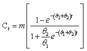(2)

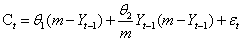
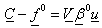
To estimate the parameters from the time series data on power consumed, the following analogue to equation (1) was used:

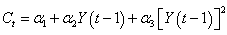(3)

We utilize two approaches; Indirect least square (ILS) and Non-linear least square (NLS) to estimate the multiple regression (3). The Indirect least square (ILS) estimate of , given by 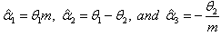are obtained. The parameters of the basic model () in (1) are identified in terms of these regression coefficients derived as:

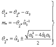(4)

Given that is fixed, the mean and variance of of the estimators given in equation (4) are derived as:

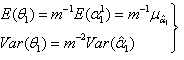(5)

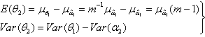(6)

Secondly, the nonlinear least squares estimation procedure suggested by[25] was introduced to overcome some of the shortcomings of the Maximum Likelihood Estimation (MLE) procedure, which itself was designed to overcome the shortcomings of the OLS procedure of[7]. Using the expression given in equation (1), that is:

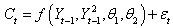
Which intrinsically, is non-linear in both parameters and exogenous variables. Suppose that we consider with then we have;

(7)

Equation (7) can be rewritten as;

(8)

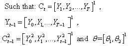Assume that is deterministic numbers and we want to estimate by linearization (Gauss- Newton) method as follows; If we are given the deterministic part of as defined in equation (8) , then we have:

With two (2) parameters and we can linearize in the neighbourhood of given;

This reduces to;

(9)

In this section, we assume that gives some correct values of in the original model with replacing ; also we set and;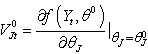

, is the 2-partial derivatives of with. Equation (9) can then be written as: ,

by rearranging and adding the error terms it reduces to;

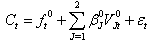(10)

Substituting in equation (10), we have:

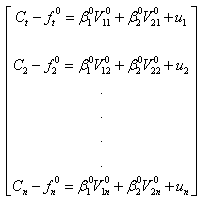(11)

In matrix form, equation (11) is given as;

(12)

If we interpret column in the linear regression case, then the least square estimate of can be written as;

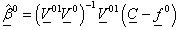(13)

Thus equation (13) gives the estimates of that minimize the sum of squares:

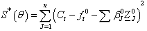(14)

Setting , we have;

(15)

This gives an improved initial estimate of parameter and would be used at the next iteration. Thus is the first revised estimate of and continues until convergence takes place; so at the iteration we have the estimate as:

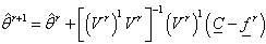(16)

The iteration continues until convergence takes place when:

Where is some small number say . Also, at every iteration, we compute to ensure that a reduction in the sum of squares has taking place; the residual mean square would be computed using:

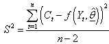, as an estimate of .

The asymptotic covariance of is; 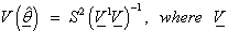is the matrix of partial derivatives defined above and evaluated at the final iteration least squares estimate of ; that is,

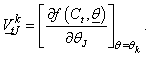Equation (15) will produced the values of the needed parameters of Bass model as also defined in (2) for Indirect least square.

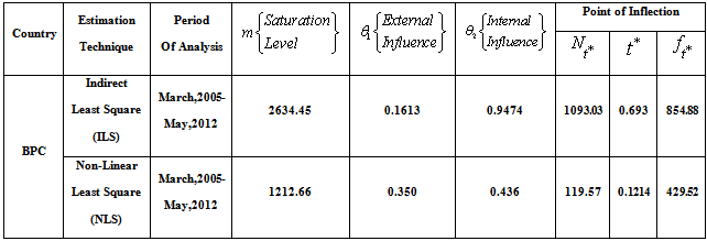
In practice, one is interested in estimating the three key parameters in equations (4) and (15) with associated statistical properties for both Indirect and Non-linear least squares respectively to be able to predict power growth in terms of power consumption, the estimates of are substituted into equation (3) to yields the S-shaped diffusion curve captured by the Bass model, for this curve,additional motivation is the point of inflection (which is the maximum penetration rate, ), which occurs when, the peak value of and the predicted time of this peak are shown to be;

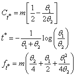(17)

3. Empirical Illustration with Reference to Botswana and Nigeria Power Consumption

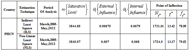
According to[17], the Bass model requires a minimum of three periods to estimate the diffusion curve; consequently in our analysis of the data collected on power output consumption in Botswana and Nigeria, the entire period March,2005-May, 2012 respectively was used for both countries to effectively see the growth point and evaluate the growth phases of power consumed, with the possibility of capturing the magnitude (m) of the consumption for an innovation as well as the general shapes of the diffusion curve with relative little input data. The relatively small data is not a disadvantage, since it had been shown that growth model can be used to describe the behaviour of random demand for a product without the sizeable data requirements typically associated with time-series models[18].

In this study, we use indirect least square (ILS) and non-linear least squares (NLS) techniques to estimate the Bass diffusion model for the power consumption data in Botswana and Nigeria, We analysed 86 point power consumption data respectively for both countries to establish the growth in consumption and estimate the external () and internal () diffusion rates and obtain the saturation point () for the periods.

Equation (2) yields curved as shown in figure 1 through 4, the diffusion curves captured by the Bass model as displayed shows an evolution over time () of the cumulative power consumption penetration () and the penetration changes per time unit i.e. . From the power consumption growth curves, in the early stages, radical innovation take place, while in the subsequent growth phases incremental innovations occurs, and eventually, saturation takes places and the power growth curve as presented in figure 1 through 4 presented some variations in the power consumption performance as a function of time. 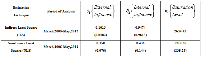It is observed that for all the methods utilized. The power consumption output (MW) for Botswana (March,2005-May,2012) and Nigeria (March,2005-May,2012) converges in most cases to the same values as showed in figure 1 through 4, indicating the power consumption saturation levels for both countries. And, comparing the values of the parameters presented in Table 1 through 4 obtained using Indirect and Non-linear least squares methods, the internal influence () using Non-linear approach have influence on Botswana power consumption pattern and it fell within the Bass benchmark of 0.38 to 0.5 according to[11]. 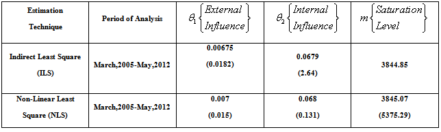However, the external influence () for both ILS and NLS fell outside the range, indicating that the rate of power consumption is only affected by consumers who are already using the power.

The Nigeria power consumption is majorly influenced by the external influences as indicated by both Indirect and Non-linear least squares (), these competitive techniques yielded the same values which is within the benchmark of 0.03 to 0.01 according to[11]. But the internal influence () for both ILS and NLS are outside the benchmark range, indicating the likelihood of power generated are not yet consumed by power subscribers due to constraints caused by internal and external factors affecting the power sector.

4. Conclusions

The parameters obtained can be used to make power consumption projection and these can be a very useful performance capacity planning for a power generation plants, estimating power unit production costs, forecasting revenue and cash flow overtime. From the managerial point of view, the extractions of the Bass diffusion parameters early in the power consumption process will be most interesting for power planning purposes, while for research purposes, the determination of the Bass diffusion parameters will be used for the validity of the diffusion model and possibly refining the model. Hence, from the power consumption policy view point, it helps in obtaining an accurate idea about the power consumption saturation level early in the consumption process, this will helps in the power consumption capacity efficient planning and projection policy.

APPENDIX A:

Table 1. Parameter estimates of the power consumption in botswana using indirect least square (1ls) and non-linear least square (nls)

Table 2. Parameter estimates of the power consumption in nigeria using indirect least square (1ls) and non-linear least square (nls)

Table 3. Computation of point of inflection for botswana power consumption (bpc)

Table 4. Computation of point of inflection for nigeria power consumption (phcn)

APPENDIX B:

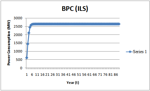Figure 1. THE diffusion Curve Captured by the Bass Model CumulativeForecast using Indirect Least Square (ILS)

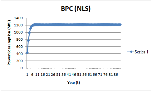Figure 2. THE diffusion Curve Captured by the Bass Model Cumulative Forecast using Non-Linear Least Square (NLS) for Power Consumption in Botswana (BPC)

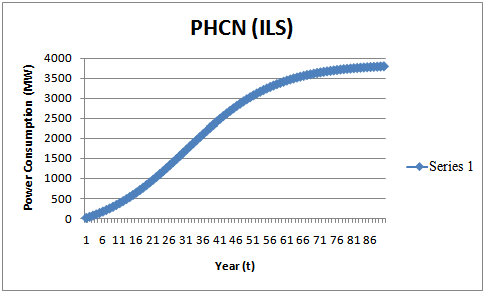Figure 3. THE diffusion Curve Captured by the Bass Model Cumulative Forecast using Indirect Least Square (ILS)

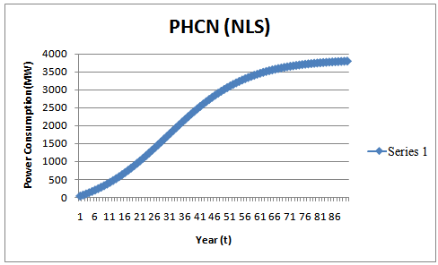Figure 4. THE diffusion Curve Captured by the Bass Model Cumulative Forecast using Non-Linear Least Square (NLS) for Power Consumption in Nigeria (PHCN)