-
Paper Information
- Next Paper
- Paper Submission
-
Journal Information
- About This Journal
- Editorial Board
- Current Issue
- Archive
- Author Guidelines
- Contact Us
American Journal of Mathematics and Statistics
p-ISSN: 2162-948X e-ISSN: 2162-8475
2013; 3(3): 95-98
doi:10.5923/j.ajms.20130303.01
Marginal Asymmetry Measure Based on Entropy for Square Contingency Tables with Ordered Categories
 Abstract
 Reference
 Full-Text PDF
 Full-text HTML
Kouji Tahata, Takuya Yoshimoto, Sadao Tomizawa
Department of Information Sciences, Tokyo University of Science, Noda City, Chiba, 278-8510, Japan
Correspondence to: Kouji Tahata, Department of Information Sciences, Tokyo University of Science, Noda City, Chiba, 278-8510, Japan.
| Email: |  |
Copyright © 2012 Scientific & Academic Publishing. All Rights Reserved.
For the analysis of square contingency tables, Tomizawa, Miyamoto and Ashihara (2003) considered a measure to represent the degree of departure from marginal homogeneity. The measure lies between 0 and 1, and it takes the minimum value when the marginal homogeneity holds and the maximum value when one of two symmetric cumulative probabilities for any category is zero. This paper proposes improvement of the measure so that the degree of departure from marginal homogeneity can attain the maximum value even when the cumulative probabilities are not zero. The proposed measure would be useful for representing the degree of departure from marginal homogeneity, especially when some asymmetry models hold as the extended marginal homogeneity model or the conditional symmetry model. Examples are given.
Keywords: Kullback-Leibler information, Measure, Power-divergence, Shannon entropy
Cite this paper: Kouji Tahata, Takuya Yoshimoto, Sadao Tomizawa, Marginal Asymmetry Measure Based on Entropy for Square Contingency Tables with Ordered Categories, American Journal of Mathematics and Statistics, Vol. 3 No. 3, 2013, pp. 95-98. doi: 10.5923/j.ajms.20130303.01.
Article Outline
1. Introduction
- Consider an
 square contingency table with the same row and column classifications. Let
  denote the probability that an observation will fall in the
  th row and
  th column of the table (
 ), and let
  and
and  denote the row and column variables, respectively. The marginal homogeneity (MH) model is defined by
  namely
  where
where  and
and  (see, for example, Stuart, 1955; Bishop, Fienberg and Holland, 1975, p.293). Let
 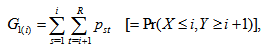 and
and 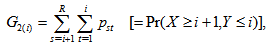 for
for  . By considering the difference between the
  and
and  , the MH model also be expressed as
 Namely, this states that the cumulative probability that an observation will fall in row category
  or below and column category
  or above is equal to the cumulative probability that the observation falls in column category
  or below and row category
  or above for
  . When the MH model does not hold, we are interested in measuring the degree of departure from MH. For square contingency tables with ordered categories, Tomizawa, Miyamoto and Ashihara (2003) proposed the measure (denoted by
  in Section 2) to represent the degree of departure from MH. The measure
  ranges between
  and
and  Also, (i)
  if and only if the MH model holds, and (ii)
  if and only if the degree of departure from MH is a maximum; that is,
  (then
(then  ) or
) or  (then
(then  ) for all
  . However, for the analysis of square contingency tables, all cell probabilities
  are positive in many cases. Thus, the measure
  may be unsuitable for such data, because the measure
  cannot attain the maximum value. So, we are now interested in the measure to represent the degree of departure from MH such that it can attain the maximum value even when each of cell probabilities
  is not zero. Yamamoto, Masumura and Tomizawa (2011) considered such a measure for nominal square table. We are now interested in proposing such a measure for ordinal square table. The purpose of this paper is to consider an improvement of measure for square contingency tables with ordered categories when all cell probabilities
  are positive.
2. Improved Measure for Marginal Homogeneity
- Consider an
 table with ordered categories. Assume that
  are positive. Let
  for
for  ; and let
  For a specified
  which satisfies
  and
and  for all
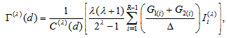
  , consider a measure defined by
 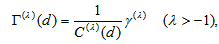 where
where 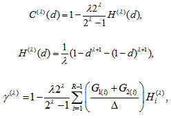 with
with 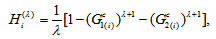 and the value at
  is taken to be the limit as
  . Thus,
 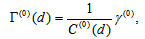 where
where 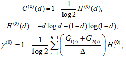 with
with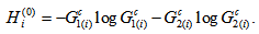 Note that
  is the diversity index proposed by Patil and Taillie (1982), which includes the Shannon entropy when
  . When
  , then
  is identical to the measure
  given by Tomizawa et al. (2003). Since
  , the minimum value of
  is
is 
 and the maximum value of it is
  or
or  (if
(if  ) when
  for all
  . So, when
  cannot attain the value 1. The proposed measure
  with
with  is modified by using modification coefficient
  such that the measure
  can attain the value
  . If all
  are positive, then
  must be taken as
  . Moreover, for each
  and a fixed
  , the measure
  has characteristics that (i)
  must lie between
  and
and  , (ii)
  if and only if the MH model holds, i.e.,
  for all
  and (iii)
  if and only if the degree of departure from MH is the largest in the sense that
  for all
  . The measure also may be expressed as, for
 where
where 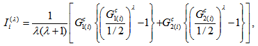 especially
 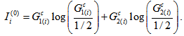 Note that
  is the power-divergence between
  and
and  (Cressie and Read, 1984) which includes the Kullback-Leibler information when
  .
. 3. Approximate Confidence Interval for Measure
- Let
 denote the observed frequency in the
  th row and
  th column of the table (
 ). Assume that a multinomial distribution applies to the
  table. The sample version of
  , is given by
  with
with  replaced by
  , where
  and
and  . Using the delta method (Bishop et al., 1975, Sec. 14.6),
 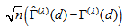 has asymptotically (as
  ) a normal distribution with mean zero and variance
 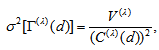 where for
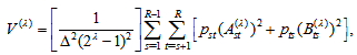 with
with 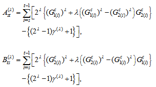 and the value of variance at
  is taken to be the limit as
  . Let
. Let  denote
  with
with  replaced by
  . Using this result, the estimated approximate confidence interval for the measure
  is obtained.
 4. Examples
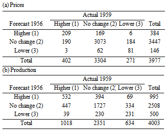
- Consider the data in Table 1, taken from Andersen (1997, p.226). These data show the forecasts for production and prices for the coming three year periods given by experts in July 1956 and the actual production figures for production and prices in May 1959 given from Danish factories. For these data, the cell probabilities
 are theoretically positive (not zero). Thus, it may be irrelevance to use the measure
  with
with  . So we should use the measure
  with
with  (for example,
  ) so that the measure can attain the maximum value 1.
|
|
 , the estimates of
  , estimated approximate standard error for
  , and approximate 95% confidence interval for
  , applied to Tables 1a and 1b.
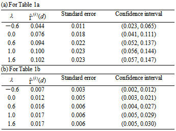
 and
and  , the estimated measure
  is
is  for Table 1a and
  for Table 1b from Tables 2a and 2b. Thus, (i) for Table 1a, the degree of departure from MH is estimated to be
  percent of the maximum degree of departure from MH and (ii) for Table 1b, it is estimated to be
  percent of the maximum. Furthermore, we see from Tables 2a and 2b that the degree of departure from MH is greater for Table 1a than for Table 1b because the values in the confidence intervals for
  are greater for Table 1a than for Table 1b.
5. Discussion
- Consider the extended MH (EMH) model defined by
 also see Tahata and Tomizawa (2008). A special case of EMH model obtained by putting
  is the MH model. When the EMH model holds, the proposed measure
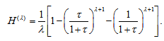
  is expressed as
  | (1) |
 For
For  fixed and
  fixed,
  increases as
  increases (or as
  decreases). Especially, when
  ,
,  is identical to
  proposed by Tomizawa et al. (2003). When the EMH model holds,
  approaches 1 as
  approaches infinity or zero. However, when the EMH model holds,
  cannot attain 1 because then
  and
and  , namely there is not the structure of
 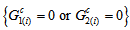 being the condition of
  . The measure
  with
with  can attain the maximum value 1 even if
  and
and  for all
  . Therefore, the measure
  with
with  rather than
  may be appropriate when the EMH model holds. Also since the probabilities
  are positive (not zero), the measure
  with
with  rather than
  would be appropriate to represent the degree of departure from the MH toward the structure of maximum departure from MH which can be defined actually.The conditional symmetry (CS) model (McCullagh, 1978) is defined by
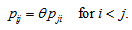 A special case of this model obtained by putting
  is the symmetry model (Bowker, 1948). If the symmetry model holds, then the MH model holds. Also if the CS model holds, then the EMH model holds. Therefore when the CS model holds, the measure
  is expressed by with
  replaced by
  . Thus by the similar reason, when the CS model holds, the measure
  with
with  rather than
  would be appropriate.