Xiaoyu Lu, Sunil Dhar
Department of Mathematics, New Jersey Institute of Technology, Newark, 07102, USA
Correspondence to: Xiaoyu Lu, Department of Mathematics, New Jersey Institute of Technology, Newark, 07102, USA.
| Email: |  |
Copyright © 2012 Scientific & Academic Publishing. All Rights Reserved.
Abstract
In adaptive dose-finding clinical trials, the strategy is to initially include only a few patients on some doses to explore the dose–response, then to allocate the dose range of interest to more patients. This reduces the allocation of patients to non-informative doses and also save the trial cost. Bayesian adaptive dose finding design has the ability to utilize accumulating data obtained in real time to alter the course of the trial, thereby enabling dynamic allocation to different dosing groups and dropping of ineffective dosing group earlier. In this research, Bayesian adaptive method was used as a new and useful approach that applies to phase II dose-finding clinical trials to evaluate safety and efficacy of the study treatment. We applied Normal Dynamic Linear Models (NDLMs) and response model in stages 1-4. Conditional probability for each parameter in the model was derived using appropriate prior distributions. Markov Chain Monte Carlo (MCMC) method is used to do the simulation. The results give clearer idea if one needs to go further to test new dose levels based on the thorough evaluation of the existing partial data. Model parameters with meaningful prior distributions and the posterior quantities are obtained to evaluate the trial results and they help to determine the optimal dose level which can be used in the phase III study. Simulations have been done for different scenarios and used to validate the model. Five thousands simulation trials were conducted to verify the repeatability of the results. The posterior probability of success for the trial is greater than 90% based on the simulation result. Comparing with the other adaptive dose finding strategy, the proposed Bayesian adaptive design are sensitive and robust to help the investigators draw conclusion as early as possible. The design can reduce sample size substantially which in turn leads to savings in cost and time.
Keywords:
Bayesian, Adaptive, Clinical Trials, Dose Finding
Cite this paper: Xiaoyu Lu, Sunil Dhar, The Application of Bayesian Adaptive Design in Clinical Trials, American Journal of Mathematics and Statistics, Vol. 3 No. 2, 2013, pp. 67-72. doi: 10.5923/j.ajms.20130302.01.
1. Introduction
Traditional frequentist statistics has had the dominant, and often exclusive, role in this scientific renaissance. The greatest virtue of the traditional frequentist approach maybe its extreme rigour and narrowness of focus to the experiment at hand, but a side effect of this virtue is inflexibility, which in turn limits innovation in the design and analysis of clinical trials. Because of this, clinical trials tend to be overly large, which increases the cost of developing new therapeutic approaches, and some patients are unnecessarily exposed to inferior experimental therapies. Biostatisticians in the drug and medical device industries are also increasingly faced with data that are highly multivariate, with many important predictors and response variables. Owing to such issues, there is increasing interest in Bayesian methods in clinical trials. Bayesian method is a dynamic process which uses information from the interim analysis and each stage to adaptively make the decision during the trial. Advances in computational techniques and power are also facilitating the application of these methods[1]. Currently Bayesian methods are increasingly being used in drug development for a wide variety of disease and conditions, from Alzheimer’s disease to obesity, diabetes, hepatitis C, etc. Bayesian statistics tries to find the probabilities of all of the parameters, using all available evidence from previous data, expert opinion, known structural relationships. Thus Bayesian inference can be updated continuously as data accumulated, and are not tied to the design chosen. In particular, the sample size need not be chosen in advance. As the result, the sample size and cost can be saved.This research reports the new design, implementation, and outcome of a Bayesian adaptive, dose-ranging trial incorporating an innovative dose finding approach to flexibly address both efficacy and safety aspect of the drug. A four-stage Bayesian adaptive design is proposed for a dose-finding study treating cancer patients. Bayesian statistics is used in the clinical trial and Gibbs sampling method will be used for the simulation.
2. Bayesian Adaptive Design and its Application in Phase IB Double Blinded Clinical Trial
The Bayesian Adaptive design is proposed to a Phase IB double blinded oncology trial treating breast cancer patients.The fluorodeoxyglucose positron emission tomography (FDG-PET) is a widely used biomarker which is most commonly known in cancer diagnosis and is used as the method to measure the efficacy response in this trial[2].FDG accumulation was measured using the standardized uptake value (SUV) as follows[3]: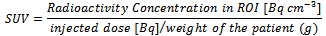 Where ROI is Region of Interest, Radioactivity concentration in the ROI was determined as the maximum average radioactivity concentration in the tissue at 55 to 60 min post-injection, corrected for calibration and decay.In this trial, a successful efficacy endpoint/response is defined as a subject has >= 20% decrease on the sum of FDG-PET uptake SUVmean and SUVmax at 7 days post-dose compared to pre-dose. A successful safety response is evaluated by adverse event and laboratory values. It is expensive to use FDG-PET scan comparing with CT/MRI in the clinical trial. The fundamental goal of the proposed adaptive design used in this trial is to reduce the sample size, to find the optimal dose efficiently, so as to save the cost and also avoid too many subjects to be exposed to wasted doses. The efficiency of this approach is increased by the use of frequent interim analysis of accumulating data. In the trial, subjects will be randomized to 6 treatment groups (corresponding to placebo, 2.5 mg, 5 mg, 10 mg, 25 mg, 50 mg doses) and three interim analyses will be performed during each stage. The use of Bayesian approach produces predictive probabilities for success in Phase III. It also yields a transparent analysis that supports quantitative decision making. The design allows the range of doses to be adaptively expanded either up or down.This is a four-stage design.Stage 1:In stage 1, only 10 mg dose and placebo will be evaluated. Eight subjects will be randomized into 10 mg group and four subjects into placebo group in a 2:1 ratio in this stage. The reason of choosing eight subjects is to make the final maximum sample size for each group to be 12. Twelve subjects per arm are calculated by sample size calculation method using historical data. Three interim analyses will be performed in each stage. For the first interim analysis, four subjects will be randomized to 10 mg group and two subjects will be randomized to placebo group. After the subjects taking the dose, the efficacy response, the sum of the SUVmean and SUVmax of FDG-PET uptake, will be measured and the safety data will be recorded. A successful response is defined as a subject has >=20% decrease on the FDG-PET uptake at 7 days post-dose compared to pre-dose, is a clinical meaningful response in treated group compared to placebo. Pr (0.2 ≤ θd | Data),θd refers to the percent of decrease on the sum of SUVmean and SUV max of FDG-PET uptake for dose d. Let θd be the mean response to dose d. d=0 for placebo and 1-5 for each dose level in the ascending order. The probability of having 0.2 ≤ θd will be evaluated. The posterior quantities will be calculated and utilized. In the first stage, θ1 is used for the mean dose response. As the next step for the second interim analysis, two more subjects will be added into 10 mg group and one subject will be randomized into placebo group. The posterior quantities will be calculated again using expanded data. If Pr (0.2≤θ1 | Data) < 0.2 for these two consecutive analyses, this dose level will be declared as futility and the study will move onto the next stage. Otherwise, two more subjects (the 7th to 8th subject for 10 mg arm) would be added. The posterior quantities will be calculated again.Given the results of those three interim analyses on efficacy, the efficacy of 10 mg group would be evaluated using the following criteria:If Pr (0.2≤ θ1| Data) <0.2 for any of two consecutive analyses, this dose level will be declared as futility. Otherwise, the dose level will be declared as non-futility.In any case, if the dose level has safety concern, the higher dose levels would not be tested in the next stage. Similarly, if the dose level is futile, the lower dose levels would not be tested in the next stage.If Pr (0.2≤ θ1 | Data) ≥ 0.8 for any of two consecutive analyses, this dose level will be declared as effective. In this case, stage 1 will be ended early and the trial will enter stage 2.Additionally, four subjects will be randomized into placebo group in stage 1. Stage 2:One of the following four actions would be taken in stage 2 based on the results in stage 1:a) If the safety is good and the efficacy is non-futile, then the next higher and the next lower dose groups (i.e., 5 mg and 25 mg) will be assessed in stage 2.b) If the safety is not good and the efficacy is non-futile, then the next lower dose group (i.e., 5 mg) will be assessed in stage 2.c) If the safety is good and the efficacy is futile, then the next higher dose group (i.e., 25 mg) will be assessed in stage 2.d) If the safety is not good and the efficacy is futile, then four more subjects will be added into 10 mg group for re-evaluation. The efficacy and safety will be re-evaluated using expanded data with the criteria a)-c) above. If the safety is still not good and the efficacy is still futile, then the trial will be ended. Otherwise, the study will enter stage 2 without anyone to be randomized into 10 mg group in the next stage.Although there may still be some subjects to be randomized into 10 mg group in stage 2, 10 mg group will not be focused in this stage, since it has been tested previously. If there were 12 subjects randomized into 10 mg group in stage 1 due to re-evaluation in case 4, there would be no subjects to be randomized into 10 mg in stage 2.If 5 mg and/or 25 mg will be tested, the randomization ratios between the new dose levels in stage 2 (i.e., 5 mg and/or 25 mg) and the old dose levels in stage 1 (i.e., placebo and 10 mg) would be 2:1. Totally eight subjects in each new dose level and four subjects in each old level will be randomized in stage 2. Similar to the procedures in stage 1, those eight subjects in the new dose levels will be randomized in three steps by 2:1:1. Three interim analyses would be done to evaluate the efficacy at the end of each step.Normal dynamic linear models (NDLMs) will be used in stage 2 and all later stages to borrow information across adjacent doses.Stages 3:Similar to stage 2, the other new dose levels (2.5 mg and 50 mg) may be tested according to the analyses in the previous stages. In stage 3, totally eight subjects in each new dose level, and two subjects in placebo and four subjects in each levels in the previous stage, will be randomized, see Table 2.2.Stage 4:If a dose level in stage 4, either 2.5 mg group or 50 mg group, is good in safety and non-futile in efficacy, four more subjects will be randomized into that dose group to make the total number of subjects to be twelve in each of these dose groups, along with 2 in the placebo group. The final tested dose level will have twelve subjects in order to be considered adequate to evaluate both efficacy and safety assessments.During the course of the trial, the dose response curve should be monitored. In case no significant response changes between the two doses have been observed, the trial should not go to the higher dose and the threshold of the response curve is assumed. The non-significant response changes can be defined as:• Posterior mean > 0.75• Difference of two posterior means for two adjacent doses is less than 0.05
3. Statistical Models Used in the Proposed Design
3.1. Response Model Used in Stage 1
Predictive probability from response model will be used to guide the decisions to terminate the trial for futility or move onto the next stage. Let θd be the mean response to dose d for response variable Y.Here,Y ~ θd + εθd ~ N(μ0, σ02), ε ~ N (0, σε 2)
3.2. Normal Dynamic Linear Models (NDLMs) in Stage 2-4
A dose-response model based on a Normal Linear Dynamic Model (NDLMs) described by West and Harrison (1997)[4] are used in this paper. NDLM is essentially a piecewise linear model and has been used in clinical trials before. It provides the necessary flexibility to encompass both monotonic and non-monotonic dose-response relationships. It can be also easily implemented in a Bayesian updating frame work. Within this framework it provides direct probabilistic statements about many features of the dose-response. An additional advantage of NDLM is the existence of analytical results for the determination of the posterior distribution of the dose-response curve. NDLMs are also used to borrow information across adjacent doses[5]. Let Yi be a generic outcome response variable and let θdi=EYi be the mean response for dose d. The following error structure is assumed for Yi,Yi ~ θdi + εdi, i = 2, 3, 4, 5,where di is the dose given to the i-th stage. It is assumed that εdi are an iid sample from N (0, σε2) and the θdi is an independent iid sample from θdi ~ N(θ, σθ2). An NDLM is used to defined with the following assumptionsθdi ~ N(μ, σθ2), i=2, 3, 4, 5, ε ~ N(0, σε2).The parameter σθ2 represent the borrowing from one dose to the neighboring doses. The drift parameter is the variance between responses at neighboring doses. The larger the value of σθ2, the less borrowing from neighboring doses. The prior distribution for the parameter σθ 2 in the NDLM is σθ2 ~ IG (a1, b1)The prior distribution for the error variance is σε2 ~ IG (a2, b2)Inverse Gamma was specified in Berry model and it is typical in Bayesian statistics. It serves as conjugate prior of the variance of the normal distribution. So it is easy to use. Under the prior specification[6]:p(σε2, σθ2, µ)=p(σε2)p(σθ2)p(μ).
4. Simulations
When developing an adaptive design, a critical step is to simulate its performance across a variety of hypothesis response pattern scenarios. In this research, Bayesian statistics is used in an adaptive dose-find clinical trial and Gibbs sampling method will be used for the simulation.In order to simulate the design, assumptions have to be made to generate data representative of each response pattern. These assumptions do not affect the design or the analysis, but they are necessary to simulate the trial results. Bayesian probability measures the degree of belief that you have in a random event. By this definition, probability is highly subjective. It follows that all priors are subjective priors. Not everyone agrees with this notion of subjectivity when it comes to specifying prior distributions. There has long been a desire to obtain results that are objectively valid. Within the Bayesian paradigm, this can be achieved by using prior distributions that are "objective" (that is, that have a minimal impact on the posterior distribution). A prior distribution is non-informative if the prior is "flat" relative to the likelihood function. Thus, a prior is non-informative if it has minimal impact on the posterior distribution of  . Many people favor non-informative priors because they appear to be more objective.The selection of the priors used in dose-response model and NDLM is based on the historical data and non - informative rule. The selection of each parameter specified in prior distribution is specified below:a) μ0 = 0.2 A successful efficacy response is defined as a subject has >= 20% decrease on the sum of SUVmean and SUVmax of FDG-PET uptake at 7 days post-dose compared to pre-dose. To obtain equal probability of positive and negative efficacy responses, we choose 0.2 as a flat prior. This will change after we have more data to bring in.b) σ0 =0.1The possibility of increasing on the SUV is very small (=0.025). If the drift effect is noticed in the data, σ0 could be adjusted to a larger one accordingly. 0.2/1.96 ≈ 0.1c) a1=a2=2Standard deviation doesn’t exist when a1=a2=2 for inverse gamma. The same approach is used when we choose μ0. The distribution is close to ‘non-informative’. The result will be data driven which fits one’s need since there is no reliable estimation.d) b1=0.0266Based on the historic data[7], the standard deviation of θ is 0.163 and the variance is 0.0266. And the mean of IG(a1, b1) is b1/(a1-1)=b1=0.0266e) b2=0.0026 The estimate of standard errors is based on the prior data with some assumption to fit our needs. According to the historic data, standard errors of SUV reduction are 0.02164 and 0.00776 in 10 mg and 25 mg groups, respectively[6].Using those two observed numbers, the variance of standard error is 0.00026 with the mean of 0. To be conservative, taking 0.0026 as the mean of IG, b2=mean*(a2-1) =0.0026 when a2=2.If over-estimated, Bayesian design would not be sensitive enough. The worst case scenario is to enroll all 76 subjects without any savings on the sample.
4.1. Simulation Results
Table 1 shows one scenario of the assumed true mean of SUV decreasing used in the simulation. Four random values are taken from SAS random function as the observed values from normal distribution with previously assigned N (0.2, 0.026) for θd1. The prior chosen for σε2 is IG (2, 0.0026). In stage 1, eight patients are assigned to the 10 mg dosing group. The simulation was done for the first interim analysis with four subjects’ values. Another four subjects’ values were simulated for the second and third interim analyses after the first interim analysis data obtained. Five thousand iterations are used in the program and the first 1000 burn-in results are discarded. The sample response data of eight subjects are shown in Tables 2. Table 3 shows additional four sample subjects added in the next stage and used to confirm the results in the previous stage. 5000 simulation trials were conducted to verify the repeatability of the simulation results. The first column is the posterior mean of θd1. The second column is the standard deviation. If posterior mean of θd1 is greater than or equal to 0.2, the tested dose level is defined to be effective. If it is less than 0.2, the tested dose level is determined to be futile. By repeating the trial for 4999 times, the rate to correctly declare the effective of 10 mg dose based on success in Table 4 is 91%. That means if the true SUV decreasing is 0.21 for 10 mg dose, the chance that one accepts the efficacy of 10 mg and go into the second stage to test 5 mg and 25 mg is 91% when safety assessment turns out to be acceptable.| Table 1. Scenario 1 - True Mean of SUV Decreasing Used in Simulation |
| | Dose Group | True Mean of SUV Decreasing Used in Simulation | | 50 mg | 0.32 | | 25 mg | 0.28 | | 10 mg | 0.21 | | 5 mg | 0.14 | | 2.5 mg | 0.10 |
|
|
| Table 2. Sample Response from Eight Patients of Each Dose Level |
| | Sample Response from the Patients (10 mg) | Sample Response from the Patients (25 mg) | Sample Response from the Patients (5 mg) | Sample Response from the Patients (50 mg) | | 0.225358 | 0.286135 | 0.1259043557 | 0.345133 | | 0.250183 | 0.304092 | 0.1190447393 | 0.318048 | | 0.196323 | 0.309638 | 0.0746307186 | 0.279937 | | 0.224806 | 0.232502 | 0.1264000144 | 0.317466 | | 0.199867 | 0.327465 | 0.0833617751 | 0.364753 | | 0.213084 | 0.274455 | 0.1406598464 | 0.348125 | | 0.203742 | 0.373889 | 0.1734469096 | 0.289752 | | 0.230214 | 0.314788 | 0.1082017321 | 0.287554 |
|
|
| Table 3. Sample Response of Additional Four Patients to Confirm the Results in Each Dose Level |
| | Sample Response from the Patients (10 mg) | Sample Response from the Patients (25 mg) | Sample Response from the Patients (5 mg) | Sample Response from the Patients (50 mg) | | 0.225358 | 0.286135 | 0.125904 | 0.345133 | | 0.250183 | 0.304092 | 0.119044 | 0.318048 | | 0.196323 | 0.309638 | 0.0746307 | 0.279937 | | 0.224806 | 0.232502 | 0.126400 | 0.317466 |
|
|
| Table 4. Results from the First Twenty Simulated Trials for 10 mg Dose Group |
| | Trial | Posterior Mean | Std Dev | Success | | 1 | 0.1986 | 0.0110 | 0 | | 2 | 0.2135 | 0.0117 | 1 | | 3 | 0.2048 | 0.0082 | 1 | | 4 | 0.2007 | 0.0090 | 1 | | 5 | 0.2205 | 0.0108 | 1 | | 6 | 0.2137 | 0.0134 | 1 | | 7 | 0.2015 | 0.0123 | 1 | | 8 | 0.1983 | 0.0088 | 0 | | 9 | 0.2093 | 0.0097 | 1 | | 10 | 0.2045 | 0.0085 | 1 | | 11 | 0.2263 | 0.0089 | 1 | | 12 | 0.2148 | 0.0135 | 1 | | 13 | 0.2043 | 0.0201 | 1 | | 14 | 0.2139 | 0.0088 | 1 | | 15 | 0.2090 | 0.0101 | 1 | | 16 | 0.2143 | 0.0104 | 1 | | 17 | 0.2013 | 0.0088 | 1 | | 18 | 0.2128 | 0.0133 | 1 | | 19 | 0.1960 | 0.0103 | 0 | | 20 | 0.2136 | 0.0105 | 1 |
|
|
| Table 5. Posterior Information for Each Dose Group |
| | Dose Group | True Mean of SUV Decreasing Used in Simulation | Posterior Mean at the end of Testing Stage | Posterior Std at the end of Testing Stage | Posterior Probability (%) of SUV Decreasing >= 0.20 | Sample Size used in the trial | | 50 mg | 0.32 | 0.308 | 0.0185 | 100.0 | 16 | | 25 mg | 0.28 | 0.297 | 0.0205 | 100.0 | 16 | | 10 mg | 0.21 | 0.227 | 0.0136 | 91.2 | 16 | | 5 mg | 0.14 | 0.125 | 0.0412 | 0.14 | 16 |
|
|
| Table 6. Operation Characteristics |
| | Scenario | Assumed Decreasing (%) at Dose Levels | Percent of Trials Selecting the Right Doses (%) | Average of the Number of Subjects Used (Saving %) | | 2.5 mg | 5 mg | 10 mg | 25 mg | 50 mg | | 1 | 10 | 14 | 21 | 28 | 32 | 91.2 | 60(16.7%) | | 2 | 10 | 14 | 15 | 20 | 25 | 73.2 | 48(33.4%) | | 3 | 2.5 | 5 | 10 | 15 | 21 | 89.2 | 33 (54.2) | | 4 | 1 | 8 | 10 | 15 | 21 | 85 | 34 (52.8) | | 5 | 0 | 3 | 10 | 15 | 20 | 72.5 | 33 (54.2) | | 6 | 0 | 0 | 0 | 0 | 0 | 100 | 28 (61.1) | | 7 | 0 | 0 | 0 | 0 | 25 | 100 | 28 (61.1) | | 8 | 0 | 24 | 30 | 30 | 30 | 100 | 43 (40.3) | | 9 | 30 | 30 | 30 | 30 | 30 | 100 | 43 (40.3) |
|
|
Similar to the simulation for 10 mg dose group, 5000 simulation trials were conducted for 5 mg. By repeating the trial for 4999 times, the rate to incorrectly declare the effective of 5 mg dose based on success in Table 5 is 0.14%. That means if the true SUV decreasing is 0.14 for 5 mg dose, the chance that one accepts the efficacy of 5 mg and go into the third stage to test 2.5 mg is 0.14% when safety assessment turns out to be acceptable. The similar simulation has been done for 25 and 50 mg dose. Since both dose levels have true responses much better than 20%, the powers to correctly detect the efficacy are as high as 100%.The values of θd1, σε2 from the first stage can be used as the prior of the second stage. The similar procedure is done for stage 2, 3 and 4. The final results of a random selected trial in simulation are showing in table 5. 2.5 mg was not tested since the 5 mg dose failed on efficacy. Assuming the safety are all good comparing with Placebo, the maximum patients need to be recruited in this scenario is 60. In case any safety issues were found in higher dose, the dose level will not go up. The sample size will be saved more.Table 6 shows operating characteristics for each dose level. In each scenario, 5000 simulated trials were conducted.
5. Conclusions
According to the simulation results, the proposed Bayesian Adaptive Designs are sensitive and robust to help investigators draw conclusion as early as possible. The designs have the ability to utilize accumulating data obtained in real time to alter the course of the trial, thereby enabling dynamic allocation to different dosing groups and dropping of ineffective dosing group earlier. The posterior probability of success for the trial is from 72-100% based on the simulation result. It increased the probability of success comparing with the other adaptive dose finding design. So it provides the better treatment to the patients. Both of the design can reduce sample size substantially which in turn leads to savings in cost and time.
ACKNOWLEDGEMENTS
We’d also like to give our special thanks to Dr. Steven Sun, Dr. Sudhakar Rao in Johnson & Johnson for their strong support and helpful suggestions.
References
| [1] | Online Available:http://en.wikipedia.org/wiki/Bayesian_probability. |
| [2] | Carol Moulton (2012). Survival analysis of PETCAM: A multicenter randomized controlled trial of PET/CT versus no PET/CT for patients with resectable liver colorectal adenocarcinoma metastatses. 2012 Gastrointestinal Cancers Symposium Meeting. |
| [3] | Paula Lindholm, Heikki Minn, et al. (1992). Influence of the Blood Glucose Concentration on FDG uptake in Cancer – A PET study. |
| [4] | Mike West, Jeff Harrison (1997), Bayesian forecasting and dynamic models (2nd ed.). New York: Springer Science + Business Media, Inc., 97-111. |
| [5] | Donald Berry, Peter Mueller, et al (1999). Adaptive Bayesian Designs for Dose-Ranging Drug Trials, fromhttp://workshop.stat.cmu.edu/berry1.pdf. |
| [6] | Martin A. Tanner (2003), Methods for the Exploration of Posterior Distributions and Likelihood Function. Tools for statistical Inference (3rd ed.). New York: Springer Science + Business Media, Inc., 211-232. |
| [7] | Garry J. Kelloff, John M. Hoffman, et al. (2005). Progress and Promise of FDG-PET Imaging for Cancer Patient Management and Oncologic Drug Development. |
 Abstract
 Reference
 Full-Text PDF
 Full-text HTML