-
Paper Information
- Next Paper
- Previous Paper
- Paper Submission
-
Journal Information
- About This Journal
- Editorial Board
- Current Issue
- Archive
- Author Guidelines
- Contact Us
American Journal of Mathematics and Statistics
p-ISSN: 2162-948X e-ISSN: 2162-8475
2013; 3(1): 32-39
doi:10.5923/j.ajms.20130301.05
A Jackknife Approach to Error-Reduction in Nonlinear Regression Estimation
 Abstract
 Reference
 Full-Text PDF
 Full-text HTML
Obiora-Ilouno H. O. 1, Mbegbu J. I. 2
1Nnamdi Azikiwe University, Awka, Nigeria
2Department of Mathematics University of Benin, Benin City Edo State, Nigeria
Correspondence to: Obiora-Ilouno H. O. , Nnamdi Azikiwe University, Awka, Nigeria.
| Email: |  |
Copyright © 2012 Scientific & Academic Publishing. All Rights Reserved.
The problems involving the use of jackknife methods in estimating the parameters of non linear regression models have been identified in this paper. We developed new algorithms for the estimation of nonlinear regression parameters. For estimating these parameters, computer programs were written in R for the implementation of these algorithms. We adopted the Gauss-Newton method based on Taylor’s series to approximate the nonlinear regression model with the linear term, and subsequently employ least square method iteratively. In the estimation of the nonlinear regression parameters, the results obtained from numerical problems using the Jackknife based algorithm developed yielded a reduced error sum of squares than the analytic result. As the number of d observations deleted in each resampling stage increases, the error sum of squares reduces minimally. This reveals the appropriateness of the new algorithms for the estimation of nonlinear regression parameters and in the reduction of the error terms in nonlinear regression estimation.
Keywords: Non- linear Regression, Jackknife Algorithm, Delete–d, Gauss–Newton
Cite this paper: Obiora-Ilouno H. O. , Mbegbu J. I. , A Jackknife Approach to Error-Reduction in Nonlinear Regression Estimation, American Journal of Mathematics and Statistics, Vol. 3 No. 1, 2013, pp. 32-39. doi: 10.5923/j.ajms.20130301.05.
Article Outline
1. Introduction
- The Jackknife is a resampling technique use for estimating the bias and standard error of an estimator and provides an approximate confidence interval for the parameter of interest. The principle behind jackknife method lies in systematically recomputing the statistic leaving out one or more observation(s) at a time from the sample set thereby generating n separate samples each of size n-1 or n-d respectively. From this new set of replicates of the statistic, an estimate for bias and the variance of the statistic can be calculated[3].[5] used linear regression analysis to examine the relationship between the Fish Age (FA) as response variable, Total Length (TL) and the Otolith Length (OL) as predictor variables. They examined dependence of FA on TL and OL using bootstrap and Jackknife algorithm.[5] used bootstrap to study linear regression model of the form
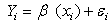 with error term
  being independent. In[5], the bootstrap errors
  are drawn with replacement from the set of estimated residuals. Response values
  are constructed as the sum of an initial estimate for
 and
and  .[6] used bootstrap method to investigate the effects of sparsity of data for the binary regression model. He discovered that the bootstrap method provided robust (accurate) result for the sparse data.[4] considers regression and correlation models, and obtain the bootstrap approximation to the distribution of least squares estimates.[2] provides algorithm for data analysis and bootstrap for the construction of confidence sets and tests in classical models which involves exact or asymptotic distribution.[14] proposes a class of weighted jackknife variance estimators for the ordinary least squares estimator by deleting any fixed number of observations at a time. He observed that the weighted jackknife variance estimators are unbiased for homoscedastic errors.[11] proposes an unbiased ridge estimator using the jackknife procedure of bias reduction. They demonstrated that the jackknife estimator had smaller bias than the generalized ridge estimator (GRE).[1] proposes Modified jackknife ridge regression estimator (MJR) by combining the ideas of GRR and JRR estimators. In their article, they proposed a new estimator named generalized jackknife ridge regression estimator (GJR) by generalizing the MJR. Their result showed that the new proposed estimator (GJR) is superior in the mean square error (MSE) than the generalized ridge regression estimator in regression analysis.
 2. Materials and Method
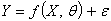
- Given a model of the form
 | (2.1) |
 are the predictor variables and the error term
  independently identically distributed and are uncorrelated.Equation (2.1) is assumed to be intrinsically nonlinear. Suppose we have a sample of n observations on the
  and
and  , then, we can write
 | (2.2) |
 | (2.3) |
 The error sum of squares for the nonlinear model is defined as
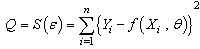 | (2.4) |
 , these estimates minimize the
  . The least square estimates of
  are obtained by differentiating (2.4) with respect to
  , equate to zero and solve for
  , this results in J normal equations:
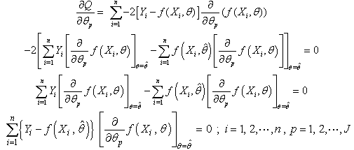 | (2.5) |
 which is the deterministic component of
  | (2.6) |
 be the initial approximate value of
  . Adopting Taylor’s series expansion of
  about
about  , we have the linear approximation
 | (2.7) |
 | (2.8) |
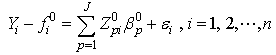
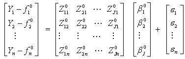
 Hence, equation (2.8) becomes
 | (2.9) |
 | (2.10) |
 | (2.11) |
 | (2.12) |
 We obtain the Sum of squares error

 | (2.13) |
 | (2.14) |
 | (2.15) |
 minimizes the error sum of squares,
 | (2.16) |
 of non-linear regression (2.1) are
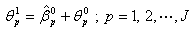 | (2.17) |
 Thus
Thus 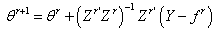 | (2.18) |
 are the least squares estimates of
  obtained at the
 iterations. The iterative process continues until
  where
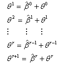
where  is the error tolerance [12][7]After each iteration,
  is evaluated to check if a reduction in its value has actually been achieved. At the end of the
  iteration, we have
  | (2.19) |
 iteration are:
 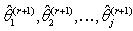 .
. 2.1. Jackknife Delete-One Algorithm for the Estimation of Non-linear Regression Parameters
- Let
 vector denotes the values associated with
  observation sets. The steps of the delete-one jackknife regression are as follows.Given randomly drawn sample of size n from a population and label the elements of the vector
  as the vector
  be the response variables,
  is the matrix of dimension
  for the predictor variables, where
  1. Omit first row of the vector
  and label remaining
  observation sets
  and
and  as the first delete-one Jackknife sample
  2. Calculate the least square estimates for nonlinear regression coefficient from the first jackknife sample;
  .3. Compute
  using the Gauss-Newton method, the
  value is treated as the initial value in the first approximated linear model.4. We return to the second step and again compute
  .At each iteration, new
  represent increments that are added to the estimates from the previous iteration according to step 3 and eventually find
  , which is
  up to
up to  .5. Stopping Rule; this iteration process continues until
 , where
  , for the values of
  from the first delete-one Jackknife estimates
  .6. Then, omit second row of the vector
  and label remaining n-1 sized observation sets
  and
and  and repeat steps 2 to 5 above for the estimate of regression coefficients
 . Similarly, omit each one of the n observation sets and estimate the non linear regression coefficients as in the step 2 to 5 above for
  alternately, where
  is Jackknife regression coefficient vector estimated after deleting of
  observation set from
  .7. Obtain the probability distribution
 of Jackknife estimates
  .8. Calculate the jackknife regression coefficient estimate which is the mean of the
  distribution[9] as;
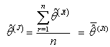 | (2.21) |
2.2. Jackknife Delete-d Algorithm for Estimation of Non-Linear Regression
- Let
 vector denotes the values associated with
  observation sets. Draw a random sample of size n from the observation set (population) and label the elements of each vector
 as the vector
  be the response variables, and
  be the matrix of dimension n × k for the predictor variables, where j=1, 2, …, k and i = 1, 2 , …, n.Step 1: Divide the sample into “s” independent group of size d.Step 2: Omit first d observation set from full sample at a time and estimate the nonlinear regression parameter
  from (n - d) remaining observation set using the least square estimate for the nonlinear regression parameter from the first delete-d sample;
  .Step 3: Compute
  using the Gauss-Newton method, the
  value is assumed as the initial value in the first approximation.Step 4: Repeat the second step and again compute
 . At each iteration, new
  represent increments that are added to the estimates
  from the previous iteration according to step 3 and eventually obtain
  up to
up to  and consequently
 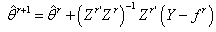 Step 5: Stopping Rule; the iteration process continues until
 , (where
 is the tolerance magnitude) and the parameters
  are computed from
  delete-d samples
  Step 6: Omit second d observation set from full sample at a time and estimate the nonlinear regression parameters
  from remaining
  observation set based on the delete-d sample; and repeat step 3 to step 5 for the second delete-d sample.Step 7: Alternately omit each d of the n observation set and estimate the parameters as
  where
where  is the jackknife regression parameter vector estimated after deletion of
  d observation set from full sample, for k =1,2,…,s; where
  , and
, and  ; where d is an integer.Step 8: Obtain the probability distribution
  of nonlinear regression parameter estimates
  .Step 9: Calculate the nonlinear regression parameter estimate
 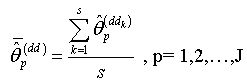 | (2.22) |
 isWhere
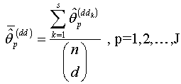 | (2.23) |
|
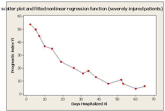 | Figure 1. Scatter Plot and Fitted Nonlinear Regression Function - Severely Injured Patients Example |
3. Results and Discussion
- Table shows the result for the parameters estimates and the error sum of squares obtained in each iteration.
|
 ) for data in Table 1


|
 for the starting values has been reduced in the first iteration and also further reduced in the second, third iterations respectively. The third iteration led to no change in either the estimates of the coefficient or the least squares
 criterion measure. Hence, convergence is achieved, and the iterations end. Table 3 shows the results of the analytical and the Jackknifes computation. The fitted regression functions for both analytical and Jackknifes delete -1 computation are:
 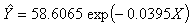 and
and  respectively. The sums of squares error for the analytical and Jackknifes computation are also shown in the table 3. Also, as the number of d observations deleted in each resampling stage increases, the error sum of squares reduces minimally.
 4. Conclusions
- We have described the Jackknife algorithm in estimation of the parameters of nonlinear regression model implementation in exponential regression model. The results obtained as shown in Tables 2 and 3 indicate that the Jackknife methods produced a minimum error sum of squares than the analytical method. We also observe that as the number of d observations deleted in each resampling stage increases, the error sum of squares reduces minimally. Hence, the Jackknife techniques yielded approximately the same inference as the analytical method with a better reduced error sum of squares.
Appendix
- Delete One Jackknife Result for the Estimates of Parameters
 y <- c(54,50,45,37,35,25,20,16,18,13,8,11,8,4,6)x <- c(2,5,7,10,14,19,26,31,34,38,45,52,53,60,65)data=cbind(y,x)initial=c(56.66,-0.03797)expo=jack(data,2,1,initial) #Run the following to view the jacknife resultstheta_0=mean(expo[,1])theta_0[1] 58.59964theta_1=mean(expo[,2])theta_1[1] -0.03958257SSE=mean(expo[,3])SSE[1] 45.73693> expo [,1] [,2] [,3][1,] 58.72515 -0.03967516 49.42362[2,] 57.69838 -0.03906341 44.59006[3,] 58.40287 -0.03950187 49.05152[4,] 59.16565 -0.03961937 42.57768[5,] 58.45181 -0.03973249 47.48378[6,] 58.66917 -0.03904419 41.73934[7,] 58.54728 -0.03931089 48.45668[8,] 58.48971 -0.03921048 47.87337[9,] 58.92722 -0.04049873 40.86874[10,] 58.60389 -0.03957958 49.45880[11,] 58.36243 -0.03902207 45.56932[12,] 59.04047 -0.04053060 35.99040[13,] 58.70595 -0.03980039 48.74806[14,] 58.44419 -0.03925252 47.21911[15,] 58.76037 -0.03989685 47.00351Deleted (= 5) E Result for the Estimates of Parameters
  y <- c(54,50,45,37,35,25,20,16,18,13,8,11,8,4,6)x <- c(2,5,7,10,14,19,26,31,34,38,45,52,53,60,65)data=cbind(y,x)initial=c(56.66,-0.03797)expo=jack(data,2,5,initial)#Run the following to view the jacknife resultstheta_0=mean(expo[,1])theta_0[1] 58.51474theta_1=mean(expo[,2])theta_1[1] -0.03953024SSE=mean(expo[,3])SSE[1] 30.75165[1,] 58.67728 -0.03959126 27.73554[2,] 58.17681 -0.03846691 38.39546[3,] 59.16003 -0.04070913 29.55899[4,] 59.68595 -0.04223456 20.55436[5,] 59.23983 -0.04121757 22.01381[6,] 59.70170 -0.04224374 18.53772[7,] 58.67701 -0.03992907 35.55294[8,] 59.17548 -0.04102820 33.88313[9,] 58.75452 -0.04008201 33.77203[10,] 59.75422 -0.04241509 20.84062
 [2994,] 59.78918 -0.04239372 16.85996[2995,] 59.39368 -0.04150764 18.60413[2996,] 58.89694 -0.04038925 32.77863[2997,] 59.84530 -0.04254249 17.11752[2998,] 58.80620 -0.04000943 30.68688[2999,] 59.26868 -0.04100269 29.02210[3000,] 58.87835 -0.04014695 28.89213[3001,] 58.37072 -0.03902467 40.60791[3002,] 59.35796 -0.04123589 29.70771[3003,] 59.01265 -0.04042930 27.88792
References
| [1] | F. SH. Batah, T. V. Ramnathan and S. D. Gore, The Efficiency of Modified Jackknife and Ridge Type Regression Estimators: A comparison, Surveys in Mathematics and its pplications 24 No.2 (2008), 157-174. |
| [2] | Beran, R., The Impact of the Bootstrap on Statistical Algorithms and Theory, Statist. Science, Mathematical Reviews (Maths Sci. Net) Vol. 18, No. 2, pp. 175-184, 2003. |
| [3] | Efron, B. and Tibshirani, R.J., An Introduction to the Bootstrap, Library of Congress Cataloging in Publication Data, CRC Press ,Boca Raton, Florida,60-82, 1998. |
| [4] | Freedman, D.A., Bootstrapping Regression Models, Annals of Statistical Statistics, Vol. 9, 2, pp. 158-167, 1981. |
| [5] | Hardle, W. and Mammen, E., Comparing Nonparametric versus Parametric Regression Fits. Annals of Statistics, Vol. 21, pp. 1926-1947, 1993. |
| [6] | Mohammed, Z. R., Bootstrapping: A Nonparametric Approach to Identify the Effect of Sparsity of Data in the Binary Regression Models, Journal of Applied Sciences, Network for Scientific Information , Asian, Vol. 8, No. 17, pp. 2991-2997, 2008. |
| [7] | Nduka, E. C., Principles of Applied Statistics 1, Regression and Correlation Analyses, Crystal Publishers, Imo State, Nigeria, 1999. |
| [8] | Neter, J., Kutner, M.H., Nachtsheim, C.J. and Wasserman, W., Fourth Edition, Mc-Grow Hill, U.S.A, pp 429-431, 531-536, 1996. |
| [9] | Obiora-Ilouno, H.O. and Mbegbu, J.I, Jackknife Algorithm for the Estimation of Logistic Regression Parameters, Journal of Natural Sciences Research, IISTE UK, Vol.2, No.4, 74-82, 2012. |
| [10] | Sahinler, S. and Topuz, D., Bootstrap and Jackknife Resampling Algorithm for Estimation of Regression Parameters, Journal of Applied Quantitative Method, Vol. 2, No. 2, pp.188-199, 2007. |
| [11] | Singh, B, Chuubey, Y. P. and Dwivedi, T.D., An Almost Unbiased Ridge Estimator. Sankhya series, 48, 342-36, 1986. |
| [12] | Smith, H. and Draper, N. R., Applied Regression Analysis, Third Edition, Wiley- Interscience, New York, 1998. |
| [13] | Venables, W. N and Smith, An Introduction to R, A Programming Environment for Data Analysis and Graphics, Version 2.6.1, pp. 1-100, 2007. |
| [14] | WU, C.F.C., Jackknife, Bootstrap and other Resampling Methods in Regression Analysis. The Annals of Statistics Vol. 14, No.4, 1261 -1295, 1986. |