-
Paper Information
- Next Paper
- Previous Paper
- Paper Submission
-
Journal Information
- About This Journal
- Editorial Board
- Current Issue
- Archive
- Author Guidelines
- Contact Us
American Journal of Mathematics and Statistics
p-ISSN: 2162-948X e-ISSN: 2162-8475
2012; 2(5): 145-152
doi: 10.5923/j.ajms.20120205.07
Discrete Burr Type Iii Distribution
 Abstract
 Reference
 Full-Text PDF
 Full-Text HTML
Afaaf A. AL-Huniti 1, Gannat R. AL-Dayian 2
1Department of Mathematics, King Abdulaziz University, Rabigh, Kingdom of Saudi Arabia
2Department of Statistics, AL-Azhar University, Cairo, Egypt
Correspondence to: Afaaf A. AL-Huniti , Department of Mathematics, King Abdulaziz University, Rabigh, Kingdom of Saudi Arabia.
| Email: |  |
Copyright © 2012 Scientific & Academic Publishing. All Rights Reserved.
In this paper, the discrete Burr type III distribution is introduced using the general approach of discretizing a continuous distribution and proposed it as a suitable lifetime model. The equivalence of continuous and discrete Burr type III distribution is established. Some important distributional properties and estimation of the parameters, reliability, failure rate and the second rate of failure functions are discussed based on the maximum likelihood method and Bayesian approach.
Keywords: Burr Type III Distribution, Discrete Lifetime Models, Reliability, Failure Rate, Maximum Likelihood Estimation, Bayes Estimation
Article Outline
1. Intro duction
- An important aspect of lifetime analysis is to find a lifetime distribution that can adequately describe the ageing behavior of the device concerned. Most of the lifetimes are continuous in nature and hence many continuous life distributions have been proposed in literature. On the other hand, discrete failure data are arising in several common situations for example:• Reports on field failure are collected weekly, monthly and the observations are the number of failures, without a specification of the failure times.• A piece of equipment operates in cycles and experimenter observes the number of cycles successfully completed prior to failure. A frequently referred example is copier whose life length would be the total number of copies it produces. Another example is the number of on/off cycles of a switch before failure occurs, see Lai and Xie[1].In the last two decades, standard discrete distributions like geometric and negative binomial have been employed to model life time data. Usually, if the discrete model is used with lifetime data, it is a multinomial distribution. This arises because effectively the continuous data have been grouped, see Lawless[2]. However, there is a need to find more plausible discrete lifetime distributions to fit to various types of lifetime data. For this purpose, discretizing popular continuous lifetime distributions can be helpful in this manner, since, it effects on speed, accuracy and understandability of the generated data using these discrete lifetime models.
1.1. Discretizing a Continuous Distribution
- A continuous failure time model can be used to generate a discrete model by introducing a grouping on the time axis. If the underlying continuous failure time X has the reliability function (RF), R (x) = P[X ≥ x ],and times are grouped into unit intervals so that the discrete observed variable is
 , the largest integer part of X, the probability mass function (pmf) of dX can be written as
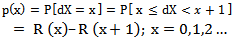 | (1) |
 this is obtained by discretizing the exponential distribution with RF
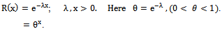 The interests in discrete failure data came relatively late in comparison to its continuous analogue. The subject matter has to some extent been neglected. It was only briefly mentioned by few scientists. Khan, Khalique and Abouammoh[3], discussed two discrete Weibull distributions (type I and type II), and suggested a simple method to estimate the unknown parameters for one of them, since the usual methods of estimation are not easy to apply. Kulasekera[4] presented approximate maximum likelihood estimators of the parameters of a discrete Weibull distribution under censoring.A discrete analogue of the normal distribution was obtained[5], that is characterized by maximum entropy, specified mean and variance, and integer support on
  . Szablowski[6], introduced new natural parameters in a formula defining a family of discrete normal distributions, where one of the parameters is closely related to the expectation and the other to the variance of that family. The discrete version of the normal and Rayleigh distributions were also proposed by Roy[7],[8] respectively. The discrete Weibull models were obtained[9], in order to model the number of cycles to failure when components are subjected to cyclical loading. In addition, some distributional properties for these models were presented.A discrete version of the Laplce (double exponential) distribution was derived by Inusah and Kozubowski[10], and discussed some of its statistical properties and statistical issues of estimation under the discrete Laplace model. The discrete Burr type XII and Pareto distribution were obtained[11], using the general approach of discretizing and then, some important distributional properties and estimation of reliability characteristics were proposed.A discrete inverse Weibull distribution was proposed[12], which is a discrete version of the continuous inverse Weibull variable, defined as X-1 where X denotes the continuous Weibull random variable. The discrete version of Lindley distribution was introduced[13], by discretizing the continuous failure model of the Lindley distribution. Also, a compound discrete Lindley distribution in closed form is obtained after revising some of its properties.A discrete generalized exponential distribution of a second type (DGE2(α,ρ)), was presented[14], which can be considered as another generalization of the geometric distribution.A discrete analog of the generalized exponential distribution (DGE(α,ρ)) was presented[15], which can be viewed as another generalization of the geometric distribution, and some of its distributional and moment properties were discussed. Burr type III distribution proposed as a lifetime model, see[16], the author discussed the distributional and the reliability properties of BurrIII(c, k).In this paper, a discrete analogue of the BurrIII(c, k) distribution is introduced, since, it plays an important role in environment and other allied sciences. It is called discrete Burr type III distribution denoted by dBurrIII(c, θ). This distribution is suggested as a suitable lifetime model to fit a range of discrete lifetime data. The rest of the paper is organized as follows: In Section 2, BurrIII(c, k) distribution is given with its reliability characteristics. The discrete analogue of BurrIII(c, k) distribution is developed with its distributional properties and reliability characteristics along with a graphical description. In Section 3, some important results on dBurrIII(c, θ) are proved. The maximum likelihood (ML) and Bayes estimations in dBurrIII(c, θ) are illustrated in detail through a simulation studies in Section 4.
2. The Model
2.1. Continuous Burr Type III Distribution
- A lifetime rv X follows the Burr type III distribution BurrIII(c, k) if its pdf is given by
 | (2) |
 | (3) |
 | (4) |
 | (5) |
2.2. Discrete Burr III Distribution
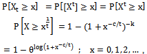
- Based on the reliability function of continuous BurrIII rv X, which is given by (3), the
 for dBurrIII(c, θ) distribution at integer points of X, is given by
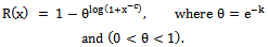 | (6) |
 is same for BurrIII(c, k) distribution and dBurrIII(c, θ) distribution at the integer points of x. Also, it is a positively skewed distribution.Now, by using (1), the pmf of the discrete Burr type III distribution with the parameters c and θ, dBurrIII(c, θ), can be define as
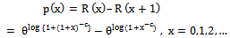 | (7) |
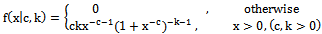
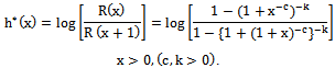
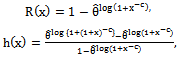
2.2.1. The Failure Rate h(x) is Given by
- The HRF or the failure rate function is given by
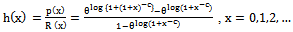 | (8) |
2.2.2. The Second Rate of Failure is Given by
- For discrete distributions, failure rate h(x) is a conditional probability with unity as its upper bound. It was pointed out that calling this the failure rate function might add to the confusion that is already common in industry that failure rate and failure probability are sometimes mixed-up[9]. To solve this problem they introduced second rate of failure
 with the same monotonicity as h(x) .For dBurrIII(c, θ) we have
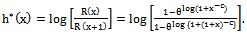 | (9) |
 for dBurrIII(c, θ) can be directly obtained from those of BurrIII(c, k) distribution, by setting
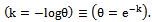
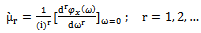
2.2.3. The rth Moment of dBurrIII(c, θ) is Given by
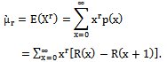 | (10) |
 of dBurrIII(c, θ) can be obtained by using (10) as follows
  | (11) |
 | (12) |
 of dBurrIII(c, θ) can be obtained by using (11) and (12) as follows
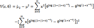 | (13) |
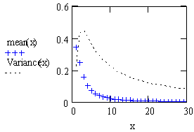 | Figure 1. Plot for the mean and the variance of dBurrIII(c, θ) |
 moment is given by
 | (14) |
 moment is given by
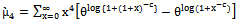 | (15) |
 of dBurrIII(c, θ) can be obtained by using (11), (12), (13) and (14) as follows
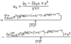 | (16) |
 of dBurrIII(c, θ) can be obtained by using (11), (12), (13), (14) and (15) as follows
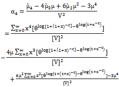 | (17) |
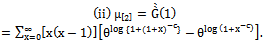
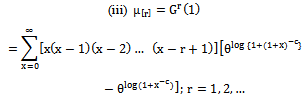
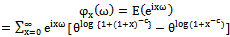
2.2.4. The Probability Generating Function  for dBurrIII(c, θ) is Given by
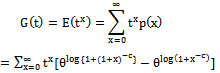 | (18) |
 | (20) |
 From (19) and (20) the variance
  of dBurrIII(c, θ) is given by
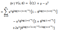 | (21) |
2.2.5. The Characteristic Function  for dBurrIII(c, θ) is Given by
 | (22) |
 then,
then,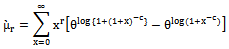 which is clearly the same result in (10).
2.3. Graphical Description
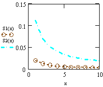
- The curves of two populations of dBurrIII(c, θ) are plotted in Fig.(2), the first curve p1(x) when (θ = .75 and c =1) and the second one, p2(x) when (θ = .25 and c = .5). The curves of the corresponding failure rate function and the second rate of failure function of dBurrIII(c, θ) are illustrated in Fig.(3) and Fig.(4), respectively. Fig.(3) demonstrate some of the possible shapes of h(x) for selected values of θ where (c=.1), the first curve h1(x) at (θ = .2) and the second one, h2(x) at (θ = 2). It is obvious that h(x) is a decreasing function. In Fig.(4) some of the possible shapes of
 represented for selected values of θ and c where
  in the first curve S1(x) and
  in the second one, S2(x).
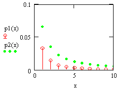 | Figure 2. Plot of the probability mass function of dBurrIII(c, θ) |
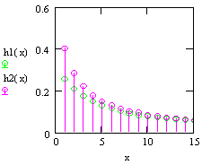 | Figure 3. Plot of the failure rate function for dBurrIII(c, θ) |
 | Figure 4. Plot of the second rate of failure for dBurrIII(c, θ) |
3. Some Results on dBurrIII(c, θ)
3.1. Result (1)
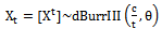
- If
 then Y=[X] ~ dBurrIII (c, θ) with
  Proof
Proof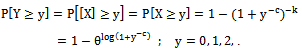 Thus, Y=[X] ~ dBurrIII (c, θ).
3.2. Result (2)
- Let
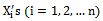 be non-negative independently and identically distributed
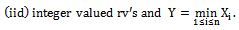 Then, Y is dBurrIII (c, θn) if and only if Xi is dBurrIII(c, θ).Proof Let
  be iid dBurrIII(c, θ), then,
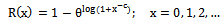 consider,
 thus,
thus, 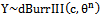 .Conversely,let
  then,
then, 
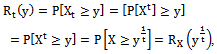
3.3. Result (3)
- If X non-negative rv and (t) is a positive number. Then,
 if and only if
  .ProofLet
  . Then,
 thus,
thus,  .Conversely, let
  , then,
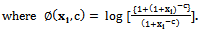
 Where,
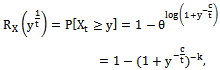 substituting
  {x will cover the whole interval
  for varying t}, we get
 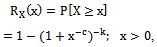 which is the RF of
  .
.3.4. Result (4)
- If
 then Y=[log(1+X-c)] ~ Geo(θ), the geometric distribution with
  .ProofConsider,
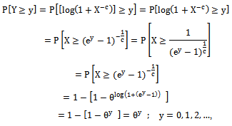 this is RF of geometric rv. Thus, Y~Geo(θ).
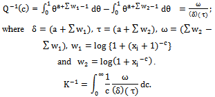
3.5. Result (5)
- If
 then
then 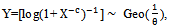 where
where ProofConsider,
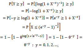 That is RF of geometric rv. Thus,
  . The following figure summarizes some of the results on dBurrIII(c, θ).
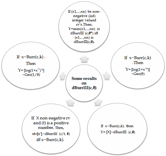 | Figure 5. Summary of some results on dBurrIII(c) |
4. Estimation of the Parameters of dBurrIII(c, θ)
4.1. Estimation of the Parameters Based on the ML Method
- Let n items be put on test and their lifetimes are recorded as
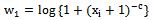
 . If these Xi's are assumed to be iid rv's following dBurrIII(c, θ), their likelihood function is given by
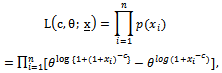 | (23) |
 | (24) |
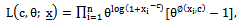
 Now, to find the two log-likelihood equations we need first to obtain the log-likelihood function which is given by
 | (25) |
4.1.1. Case I (c is Known and θ is Unknown)
- In this case, the MLE of the unknown parameter θ is
 that is the solution of the following likelihood equation, with an observed sample this equation can be solved using an iterative numerical method.
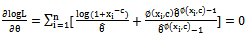 | (1) |
 and
and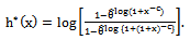
4.1.2. Case II (c and θ are Unknown)
- In this case, the solution of the following likelihood equations provide the MLE`s of the unknown parameters θ and c, which are denoted by
 respectively. With an observed sample these equations can be solved using an iterative numerical method.So those, the first derivatives with respect to θ and c, of the log-likelihood equation (25), are given by
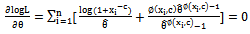 | (1) |
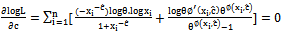 | (2) |
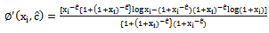 By using numerical computation, the solution of these normal equations will provide the MLE of θ and c.The MLE`s of the reliability, the failure rate and the second rate of failure functions are obtained based on the invariance property of the ML, respectively as follows
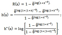
4.2. Estimation of the Parameters based on Bayesian Approach
4.2.1. Case I (c is Known and θ is Unknown)
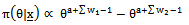
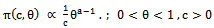
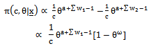
- Assume that the prior knowledge of θ is adequately represented by beta distribution with parameters (a) and (1) then the pdf of the prior density of θ is given by
 | (26) |
 | (27) |
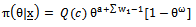 | (28) |
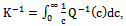
 by integrating (27) over θ leads to:
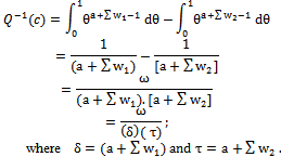 | (29) |
 distributed as followes:
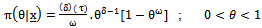 | (30) |
 | (31) |
 , the highest post estimate (HPE) of the parameter θ is given by
 | (32) |
 | (33) |
 | (34) |
 in order to get a well known form for the posterior density of the new parameter
  then
then  will be at the following form
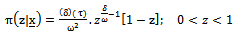 which means that,
  . Assuming a squared-error loss function and informative prior, the bayes estimate of the parameter
  is given by
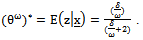 | (35) |
 the highest post estimate (HPE) of the parameter
  is given by
 | (36) |
 is givenby
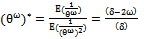 | (37) |
 is given by
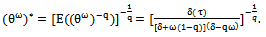 | (38) |
4.2.2. Case II (c and θ are Unknown)
- Assume that: c is distributed as a non-informative prior, θ is distributed as beta distribution where, c and θ are independent.The joint prior density of c and θ can be written as follows:
 | (39) |
 | (40) |
 ,
,  The joint posterior density (40) can be rewritten as follows
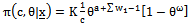 | (41) |
5.Conclusions
- The purpose of this paper is to explore a new lifetime distribution suitable for modeling discrete data, that was achieved by applying the general approach of discretizing a continuous distribution on the continuous model of Burr type III in order to introduce the discrete version of it, which is called discrete Burr type III distribution dBurrIII(c, θ). In this paper, we carry out a theoretical study of the obtained distribution discussing its distributional properties and reliability characteristics along with a graphical description. Also, we obtained and proved some important results on dBurrIII(c, θ). In addition, estimation of the parameters is discussed based on the maximum likelihood method and Bayesian approach.
ACKNOWLEDGEMENTS
- The author wishes to gratefully acknowledge the referees of this paper who helped to improve the presentation.