M. A. El-Damcese , N. S. Temraz
Department of Mathematics, Faculty of Science, Tanta University, Tanta, Egypt
Correspondence to: M. A. El-Damcese , Department of Mathematics, Faculty of Science, Tanta University, Tanta, Egypt.
| Email: |  |
Copyright © 2012 Scientific & Academic Publishing. All Rights Reserved.
Abstract
This paper presents a mathematical model for performing availability and reliability analysis of a parallel repairable system consisting of n identical components with degradation facility and common-cause failures. In addition, system repair time is assumed to be arbitrarily distributed. Markov and supplementary variable techniques are used to develop equations for the model. As an illustration, system of four-identical/repairable components is analysed.
Keywords:
Availability/Reliability Analysis, Mean Time to Failure (MTTF), Repairable Parallel System, Degradation Facility, Common-Cause Failure, Non-Markovian Process, Supplementary Variable Method
1. Introduction
Markov chain is a stochastic process that have a finite states at time t under consideration that the chain runs only through a continuous time, the basic assumption of Markov chain is the transition from the current state of the system is determined only by the present state and not by previous state or the time at which it reached the present state[1].Parallel can be used to increase the reliability of a system without any change in the reliability of the individual components that form the system. The probability of failure or unreliability for a system with n statistically independent parallel components is the probability that 1 fails and component 2 fails and all of the other components in the system fail. Therefore, in a parallel system, all n components must fail for the system to fail[2]. The problem of evaluating the availability and reliability of the parallel system has been the subject of many studies throughout the literature[3-6].It is observed that in the field of reliability, failures play a vital role. Many researchers[7-9] define different types of failures. In real systems, we cannot neglect the effect of various failures such as major failure, catastrophic failure, minor failure, common-cause failure, and so on.It is a common knowledge that redundancy can be used to increase the reliability of a system without changing the reliability of the individual unit that forms the system. It has been realized that in order to predict realistic reliability and availability of parallel systems the occurrence of common-cause failure must be considered. A common-cause failure is defined as the failure of single component ormultiple components due to a single common-cause[10]. Some of the common-cause failure may occur due to many reasons such as wrong designing of equipment during design phase, high temperature of computer chips, and so on. Most reliability models assume that the up and down times of the components are exponentially distributed. This assumption leads to a Markovian model with constant transition rates. The analysis in such cases is relatively simple and the numerical results can be easily obtained. The assumption is often valid for the up time but the down times are likely to have non-exponential distribution. When the components are independent, the steady-state results are not affected by the shape of the distribution. If the distributions cannot be represented by a single exponential form then the process becomes non-Markovian and different techniques are required for system solution. In this paper, we use the supplementary variable method. This method is used to convert non-Markov process into a Markov process by redefinition of the state space[11].By using the supplementary variable method, we can readily obtain all differential equations in terms of the state transition diagram of the model. However, it is still difficult to solve these differential equations because they usually involve some functions to be determined if there are at least two hazard rate functions involved in one of the equations. In the traditional systems, the units of the system have only two states up and down. However, in many situations the units of the system can have finite number of states. In this paper, we consider that each component of the system has three states: up, degraded, and down. The transition from up state to degraded state represents a partial failure and the transition from up state to down (failed) state or from degraded state to down (failed) state represents a complete failure.In[12], stochastic analysis of a repairable system with three units and two repair facilities was introduced. In[13], reliability characteristic of cold-standby redundant system was introduced. In[14], some reliability parameters of a three state repairable system with environmental failure were evaluated. In[15], human error and common-cause failure modelling was established for a two-unit multiple system. In[16], reliability modeling of 2-out-of-3 redundant system is introduced subject to degradation after repair. In[10], Stochastic analysis of a non-identical two-unit parallel system with common-cause failure using GERT technique. The model considered in the present paper generalizes the models discussed in literature.In this paper, we construct a mathematical model for a system consists of n repairable and identical components connected in parallel and each component has three states: up, degraded, and down. Each component of the system has three types of failures. All failures and repair rates are constant and the repaired component is good as new. The system at any working state can completely fail due to a common-cause failure with constant failure rate and in this case the system will go to the critical case c. We assume that the repair time, when the system fails due to a common-cause failure, follows general distribution. We also introduce a numerical example to illustrate the computation of steady-state availability, reliability function, and mean time to failure of a system consists of 4 components. 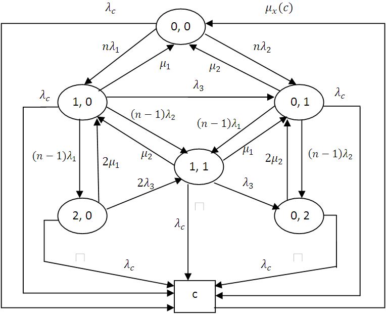 | Figure 1. State-space diagram |
2. Model Description
We consider that the system consists of n components connected in parallel and these components are identical and repairable. At time t = 0, the system is operable and it fails when all components completely fail or it fails due to common-cause failure and in this case the system goes to the critical case c. Each component has three states: up, degraded, and down and each component fails with three types of failures. All failures are statistically independent. All failures and repair rates are constant except for the repair rate from the critical case which will be not constant. So, this process is non-Markovian and we will use the supplementary variable method to convert it into Markovian process. By using supplementary variable method, we can construct the differential equations associated with the model. The state-space for the model is shown in Figure 1.
2.1. Notations
 : the constant failure rate of the unit when it goes from up state to degraded state.
 : the constant failure rate of the unit when it goes from up state to down state.
 : the constant failure rate of the unit when it goes from degraded state to down state.
 : the constant failure rate of the system when it fails due to a common-cause failure.
 : the constant repair rate of the unit from degraded state to up state.
 : the constant repair rate of the unit from down state to up state.
 : the repair rate of the failed system when it fails due to common-cause failure and the distribution of the elapsed repair time, x, is general.
 : the probability that the system is in state (i, j) at time t, where i is the number of degraded units and j is the number of failed units.
 : the Laplace transform of the probability
 .
. : the probability that the system is in the critical state c at time t and the elapsed repair time is x.
 : the steady-state probability of being in state (i, j).n : the total number of components in the system
2.2. State Probabilities
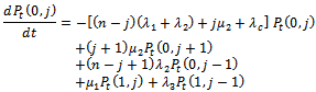
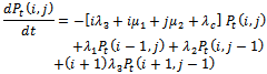
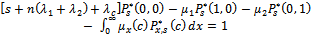
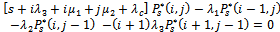
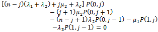
By probability and continuity arguments, the difference- differential equations for the stochastic process which is continuous in time and discrete in space are given as follows.For 
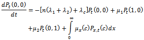 | (1) |
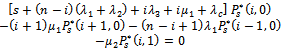
For 
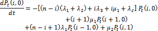 | (2) |
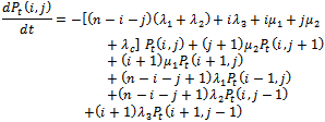
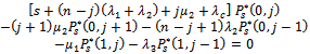
For 
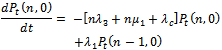 | (3) |
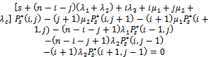
For 
 | (4) |
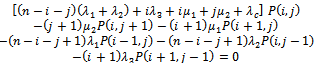
For 
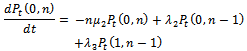 | (5) |
For
 | (6) |
For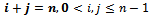
 | (7) |
For the critical case c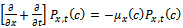 | (8) |
Boundary condition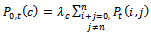 | (9) |
Initial conditions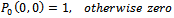
2.3. System Availability Analysis
To solve the previous mathematical model (1)-(9) for a given value of n, we will take Laplace transform of the equations from (1) to (9) and use the associated initial conditions. Hence, we obtain the following system of equations.For
 | (10) |
For 
 | (11) |
For
 | (12) |
For 
 | (13) |
For
 | (14) |
For 
 | (15) |
For 
 | (16) |
For the critical case c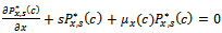 | (17) |
The boundary condition becomes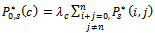 | (18) |
Solving differential equation (17), we get the following resulting expression | (19) |
Thus, from equation (18), we have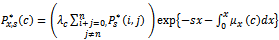 | (20) |
Now, substituting from equation (20) into the following integration, we have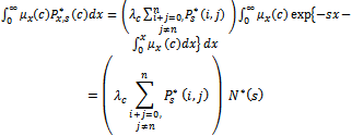 | (21) |
where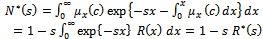 | (22) |
where  is the Laplace transform of the reliability function of the random variable X. The availability function can be obtained by taking the inverse of Laplace transform as follows.
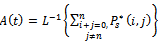 | (23) |
2.4. System Reliability and Mean Time to Failure
To obtain the reliability function of model (1)-(9), we assume that all failed states are absorbing states and set all transition rates from these states equal to zero. We also consider that 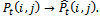 The reliability function can be obtained by taking the inverse of Laplace transform as follows.
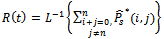 | (24) |
The mean time to system failure (MTTF) can be obtained from the following relation.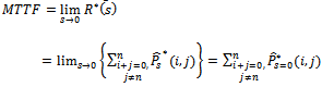 | (25) |
2.5. System Steady-State Availability
Now, to obtain the steady-state availability, we consider that: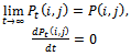 Equations (2)-(8) reduce to equations (26)-(32) respectively.For
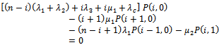 | (26) |
For 
 | (27) |
For 
 | (28) |
For 
 | (29) |
For 
 | (30) |
For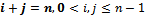
 | (31) |
For the critical case c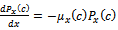 | (32) |
The sum of all probabilities equals to one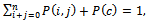 | (33) |
where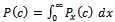 | (34) |
The boundary condition becomes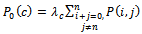 | (35) |
Solving equation (32), we get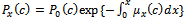 | (36) |
Substituting from equations (35) and (36) into equation (34), we get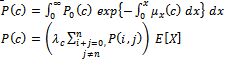 | (37) |
The steady-state availability probability can be obtained from the following relation.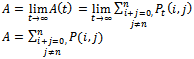 | (38) |
3. Numerical Example
In this example, we will apply the introduced mathematical model (1)-(9) for n = 4 and determine steady-state availability, reliability function, and mean time to failure of this model.In this case for (n = 4), the working states are: (0, 0), (1, 0), (0, 1), (2, 0), (0, 2), (1, 1), (3, 0), (0, 3), (1, 2), (2, 1), (4, 0), (3, 1), (1, 3), (2, 2), and the failed states are: (0, 4), (c).To obtain the reliability function, we consider that all failed states are absorbing states in the model (1)-(9), and we consider the following data:  Using numerical solutions with MAPLE program, we can solve the resultant system of equations by using equation (24) and the results are shown in Figure 2. Also, we obtain the mean time to failure by using equation (25) and the mean time to failure (MTTF) versus the common-cause failure rate
  and
and are shown in Figure 3 and Figure 4, respectively.
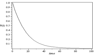 | Figure 2. Reliability function R(t) versus time |
Now, We consider that the random variable X follows Gamma distribution with parameters , hence the expected value of X will be given by
  and then we substitute in equation (37). Using the same data given in reliability, we can solve the system of equations from (26) to (31), equation (33), and equation (37) by using MAPLE program and get the steady-state availability probability by the aid of equation (38). The results for the steady-state availability probability A versus the common-cause failure rate
 and
and  are shown in Figure 5 and Figure 6, respectively.
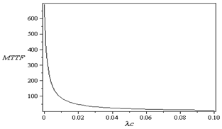 | Figure 3. MTTF versus |
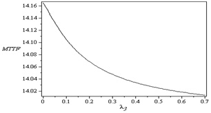 | Figure 4. MTTF versus  |
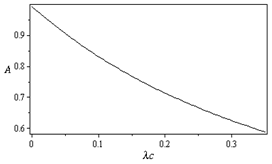 | Figure 5. Steady-state availability probability A versus  |
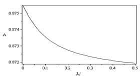 | Figure 6. Steady-state availability probability A versus  |
4. Conclusions
The main objective for this study was to offer a methodology for analysing parallel repairable system subject to degradation, common-cause failures, and general repair rate. The problem of evaluating the availability and reliability depending on the size of the parallel system was formulated in a set of first order linear differential equations form, which seems convenient for computation with software packages like Maple. Numerical solutions based on Runge-Kutta and Laplace Transform methods were used in this model to evaluate the state probabilities from the set of first order linear differential equations. Tractable solutions were found for the repairable parallel system of 4-component and 16-state. The results obtained in this paper can be applied to similar models.
References
| [1] | Birolini, A. Reliability Engineering: Theory and practice. Springer-verlag, 5th Edition , (2007) |
| [2] | Xie, M., Yuan-Shun, D., and Poh, K. Computing Systems Reliability: Models and Analysis. Kluwer Academic, New York (2004) |
| [3] | Kolowrocki, K. Limit reliability functions of some non-homogeneous series-parallel and parallel-series systems, Journal of Reliability Engineering & System safety, 46(2), 171-177(1994) |
| [4] | Pan, Z. and Nonaka, Y. Importance analysis for the system with common cause failures, Journal of Reliability Engineering & System safety, 50(3), 297-300 (1995) |
| [5] | Ebeling, C. E. An Introduction Reliability and Maintainability Engineering, Tata McGraw-Hill Education, New York (2000) |
| [6] | Kwiatuszewska-Sarnecka, B. A remark on of limit reliability function of large series-parallel systems with assisting components, Journal of Applied Mathematics and Computation , 122(2), 155-1177 (2001) |
| [7] | Gupta, R., Tyagi, P.K. and Kishan, R. A two-unit system with correlated failures and repairs, and random appearance and disappearance of repairman. International Journal of Systems Sciences, 27(6), 561-566 (1996) |
| [8] | Lam, Y. Calculating the rate of occurrence of failures for continuous time Markov chains with application to a two-component parallel system. Journal of Operational Research Society, 46, 528-536 (1995) |
| [9] | Sim, S.H. and Endrehyi, J. A failure repair model with minimal and major maintenance. Journal of IEEE Trans. on Reliability, 55(1), 134-140 (2006) |
| [10] | Sridharan, V. and Kalyani, T.V. Stochastic analysis of a non-identical two-unit parallel system with common-cause failure using GERT technique. Journal of Information and Management Sciences, 13(1), 49-57 (2002) |
| [11] | Singh, C. and Billinton, R. System Reliability Modelling and Evaluation. Hutchinson educational publishers, London (1977) |
| [12] | Wei, L., Attahiru, S.A. and Yiqiang, Q.Z. Stochastic analysis of a repairable system with three units and two repair facilities. Journal of Microelectronics Reliability, 38(4), 585-595 (1998) |
| [13] | Agarwal, S.C., Mamta S., and Shikha, B. Reliability characteristic of cold-standby redundant system, International Journal of Research and Reviews in Applied Sciences, 3(2), 193-199 (2010) |
| [14] | Sachin, K. and Anand, T. Evaluation of some reliability parameters of a three state repairable system with environmental failure, International Journal of Research and Reviews in Applied Sciences, 2(1), 96-103 (2009) |
| [15] | El-Damcese, M.A. Human error and common-cause failure modelling of a two-unit multiple system, Journal of Theoretical and Applied Fracture Mechanics, 26, 117-127 (1997) |
| [16] | Chander, S. and Singh, M. Reliability modeling of 2-out-of-3 redundant system subject to degradation after repair, Journal of Reliability and Statistical Studies, 2(2), 91-104 (2009) |
 Abstract
 Reference
 Full-Text PDF
 Full-Text HTML