1. Introduction

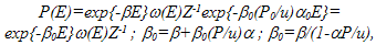
In[1] the generalization of Boltzmann factor exp{-β₀E} was introduced in the following form:

(1)

It is supposed there that the intensive parameter (return temperature, chemical potential, etc.) fluctuates. These fluctuations evolve on a long time scale. Locally, in some spatial area (cell) where β is approximately constant, the system is described by usual Boltzmann-Gibbs statistics with ordinary Boltzmann factor exp{-βE} where E is the energy a microstate associated with each cell. On a long time scale it is necessary to take into account fluctuations of β. Superposition of two statistics (that of β and that of exp{-βE}) which therefore and refers to as "superstatistics" is derived. This formalism is successfully applied to the description of fully developed hydrodynamic turbulence, defect motion in convection states, the statistics of cosmic rays and other metastable and nonequilibrium phenomena. The special case of these superstatistics, at function f, reduces to gamma- distribution, appears in the nonextensive statistical mechanics[2,3], describing a number of the physical phenomena which are not satisfactory described by Boltzmann-Gibbs statistics (for example, long-range many body systems, systems with memory, many phenomena in nuclear physics, astrophysics, geophysics, ecology, the social – communities and other complex systems). In the present work the superstatistics as (1) (together with its generalization) is obtained starting from nonequilibrium thermodynamics which as a thermodynamic variable contains a lifetime of statistical system[4,5], Section 2.

2. System Lifetime and Lifetime Distribution

Characterizing the nonequilibrium state by means of an additional parameter related to the deviation of a system from the equilibrium (field of gravity, electric field for dielectrics etc) was used in[6]. In the present paper we suggest a new choice of such an additional parameter as the lifetime of a physical system which is defined as a first-passage time till the random process y(t) describing the behaviour of the macroscopic parameter of a system (energy, for example) reaches its zero value. The lifetime is thus a random process which is slave (in terms of the definitions of the theory of random processes[7]) with respect to the master process y(t),

(2)

The characteristics of Γ depend on those of y(t). Introducing Γ means effective account for more information than merely in linear terms of the canonical distribution. It is important to make clear a physical interpretation to the definition (2). So, the lifetime is related to the period of stable existence of a system, its time of dwelling within the homeokinetic plateau whose distribution was related in[8] to the entropic and information parameters of a system, its response to internal and external influences, its stability and adaptation facilities. The states of a system within the homeokinetic plateau are characterized by the mutual compensation of the entropic effects related to the energy dissipation and by the effects of negative entropy determined by the existence of the negative feedbacks. When the system exits out of the limits of the plateau unstable structures and sharp qualitative changes in the behaviour of the system arise. We assume that the existence and the magnitude of finite lifetime is related to the deviation of the system from the equilibrium. The solution to the lifetime problem stands close to the problem of Kramers[9] (overcoming the potential barrier).

In the works on statistical physics similar definitions of thermodynamic values are encountered. For example, in[10]: "Any function B(z) of dynamic variables (z=q₁,…,q_N, p₁,…,p_N), having macroscopical character, by definition is random internal thermodynamic parameter". In[6] all values dependent on z concern are treated in this way. The fact that a lifetime (2) Γ(z) is the function of z, is obvious from the equations for distribution of a lifetime in Markov model, which are related to the equation the z-dependent density of distribution. Evidently it is visible from a situation when one considers as system some volume with gas in which all molecules are located on its borders with the velocities directed outwards. Then a lifetime is finite. For other configuration of coordinates and pulses a lifetime will be another. To validate the choice of lifetime as thermodynamic value one can ressort to the method of nonequilibrium statistical Zubarev operator (NSO)[11] which is interpreted in[12] as averaging of quasiequilibrium (relevant) the statistical operator on distribution of lifetime of the system. Then at p_q(y)=εexp{-εy}

(3)

The entropy production operator[11] is equal σ(t-u, -u)=dlnρ_q(t-u, -u)/du. If σ(t-u, -u)≈σ(t) or σ(t-u,-u)≈σ(t) has weak u-dependence then equality (3) acquires a form lnρ(t)=lnρ_q(t,0)+ <σ(t)>ε ^-1=lnρ_q(t,0)+<σ(t)><Γ>, as in interpretation[12] ε ^-1= <Γ>=0> is average lifetime. We shall note, that such distribution is received in[13]. Then a relation (3) in nonequilibrium thermodynamics with lifetime as thermodynamical parameter is replaced with expressions (5)-(6), or, in more general form, lnρ(t) = lnρ_q(t,0) + ln[Z(β)/Z(β,γ)]-γΓ, where ρ = exp{-βE-γΓ}/Z(β,γ); ρ_q = exp{-βE}/Z(β) (in (5) instead of <Γ>(dlnρ_q(t-y₁,-y₁)/dt) stand the random value Γ and Lagrange multiplier γ in: γΓ+lnZ(β,γ)/Z(β)). That is, averaging on distribution of lifetime in Zubarev NSO is replaced with use of a random variable of lifetime, - there lays essential difference of distribution (5) - (6) from (3) and from results of works[11,13].

The value Γ_x in (2) it is time before degeneration, destructions of the system. From the theory of the random processes it follows that existence and finiteness of the lifetime Γ value is related to the presence of stationary states, which physically corresponds to the existence of stationary structures. Complex functional and hierarchical relations of real systems correspond to the analogous between livetimes determining evolutionary processes as sequence of transitions between various classes of the system states. In contrast to the traditional representation about time as about something changeable, lifetime acts as result of existence of stable stationary structures. It depends on external influences on system and from internal interactions in it.

In termostatics it is supposed, that any isolated thermodynamic system eventually reaches an equilibrium state and never spontaneously leaves it. However the assumption of a possibility of fluctuations in system (i.e. random deviations of internal parameters from their equilibrium values) contradicts main principles termostatics. We shall replace the assumption of a system remaining in the basic (equilibrium) state for an infinite long time at its isolation from influence of environment with a more physical assumption (corresponding also to the statistical description) about an opportunity of a system leaving this state and destruction, degeneration of the system under influence of internal fluctuations. The open system is considered, dynamical values under influence of interaction with an environment become random; probably only macroscopical description.

The distribution for lifetime Γ (2) generally depends on macroscopical value y(t) of the master process with respect to Γ. Let us suppose that the process y(t)=E is the energy of a system (equivalently one could choose the particle number, pulse etc). Gibbs equilibrium distribution for microcanonic probability density in phase space z corresponds to a condition of equiprobability of all possible microstates compatible with the given value of a macrovariable. We shall assume, that transition of system in a nonequilibrium condition breaks equality of probabilities, characteristical for an equilibrium case. One introduces additional observable macroparameter, thus extending the phase space (containing additional degenerate, absorbing states). We shall assume validity of a principle of equal probabilities for the extended phase space divided into cells with constant values (E, Γ) (instead of phase cells with constant values E). The standard procedure (e.g.[14]) allows one to write down the relation between the distribution density P(E,Γ)=p_EΓ(x,y) and microscopic (coarse-grained) density r(E,Γ)

(4)

The structure factor ω(E) is thus replaced by ω(E,Γ) - the volume of the hyperspace containing given values of E and Γ. If m(E,Γ) is the number of states in the phase space which have the values of E and Γ less than given numbers, then ω(E,Γ)=d²m(E,Γ)/dEdΓ. It is evident that ∫ω(E,Γ=y)dy= ω(E). The number of phase points between E,E+dE; Γ,Γ+dΓ equals ω(E,Γ)dEdΓ. We make use now of the principle of equiprobability applied to the extended cells (E,Γ).

Using a maximum-entropy principle[15], it is possible to write down expression for microscopic (but coarse-grained) density of probability in the extended phase space

(5)

where

(6)

is the partition function, β and γ are Lagrange multipliers satisfying the equations for the averages

(7)

Let us underline the principal features of the suggested approach.

1. We introduce a novel variable Γ which can be used to derive additional information about a system in the stationary nonequilibrium state. We suppose that Γ is a measurable quantity at macroscopic level, thus values like entropy which are related to the order parameter (principal macroscopic variable) can be defined. At the mesoscopic level the variable Γ is introduced as a variable with operational characteristics of a random process slave with respect to the process describing the order parameter.

2. We suppose that thermodynamic forces related to the novel variable can be defined. One can introduce the “equations of state” β(,<Γ>), γ(,<Γ>). Thus we introduce the mapping (at least approximate) of the external restrictions on the point in the plane β, γ.

3. We suppose that a “refined” structure factor ω(E,Γ) can be introduced which satisfies the condition ∫ω(E,Γ=y)dy= ω(E) (ordinary structure factor). This function (like ω(E)) is the internal (inherent) property of a system. At the mesoscopic level we can ascribe to this function some inherent to the system (at given restrictions (β₀,g₀)) random process. The structure factor has the meaning of the joint probability density for the values E,Γ understood as the stationary distribution of this process. Provided the “reper” random process for the point (β₀,g₀), one can derive therefrom the shape of the structure function. If we model the dependence of the system potential of the order parameter by some potential well, the lifetime distribution within one busy period and probabilities ω(E,Γ) can be viewed as distributions of the transition times between the subset of the phase space (possibly of the fractal character) corresponding to the potential well, and the subset corresponding to the domain between the “zero” and the “hill” of the potential where from the system will roll down to the zero state. To determine the explicit form of Г (at (β₀,g₀)) the algorythm of the asymptotic phase coarsening of complex system is used (Section 3).

4. It is supposed that at least for certain classes of influences the resulting distribution has the form (5), (6), that is the change of the principal random process belongs to some class of the invariance leading to this distribution which explains how one can pass from the process in the reper point (β₀,g₀) (for example, in equilibrium when g=0 and β=1/k_BT) to a system in an arbitrary nonequilibrium stationary. The thermodynamic forces should be chosen so that the distribution lead to new (measurable) values of (,<Γ>).

3. Distribution for Nondisturbanced Lifetime

If γ=0 and β=β₀=(k_BT_eq)^-1, where k_B is the Boltzmann constant, T_eq is the equilibrium temperature, then the expressions (5-6) yield the equilibrium Gibbs distribution. One can thus consider (5-6) as a generalization of the Gibbs statistics to cover the nonequilibrium situation. Such physical phenomena as the metastability, phase transitions, stationary nonequilibrium states are known to violate the equiprobability of the phase space points. The value γ can be regarded as a measure of the deviation from the equiprobability hypothesis.

Of coarse, the thermodynamic description itself is supposed to be already coarse-grained. To get the explicit form of the Γ distribution we shall use the general results of the mathematical theory of phase coarsening of the complex systems[16], which imply the following distribution of the lifetime for coarsened random process:

(8)

for one class of the stable states and the Erlang density

(9)

in the case of several (n) classes of the ergodic stable states. The values Γ₀ and Γ_0i are averaging of the residence times and the degeneracy probabilities over stationary ergodic distributions (in our case - Gibbs distributions). The physical reason for the realization of the distribution in the form (8-9) is the existence of the weak ergodicity in a system. Mixing the system states at big times will lead to the distributions (8-9). As we note in Section 2, the structure factor ω(E,Γ) has a meaning of the joint probability density of values E,Γ. For the distributions (8), (9) the functions ω(E,Γ) from (4), (6) take on the form:

(10)

for the relations (8) and (9) respectively. Substituting into the partition function yield

(11)

for (8) and (9), where Z(β)=∫ω(E)exp{-βE}dE is the Gibbs partition function. For n=2, Z(γ)=P₁/(1+γΓ₁₀)+P₂/(1+γΓ₂₀); Γ_k0 =1/(-s_k)), k=1,2, where s_1,(2)= -(Λ₁₁+Λ₂₂)/2 + (-)[(Λ₁₁ + Λ₂₂)²/4-Λ₁₁Λ₂₂+Λ₁₂Λ₂₁]^1/2; P₁=(Γ₂₀-Γ₁₀Γ₂₀b)/(Γ₂₀-Γ₁₀); P₂= (Γ₁₀-Γ₁₀Γ₂₀b)/(Γ₁₀-Γ₂₀); b=μ₁(Λ₂₂+Λ₂₁)+μ₂(Λ₁₁+Λ₁₂); μ₁+μ₂= 1, Λ_kj are the transition intensities between the classes of states; μ_k is the probability of the initial state belonging to the k-th ergodicity class.

We have from (6)-(7) and (10) when

(12)

that is γ is the difference between the inverse lifetimes of the open system 1/Γ_g and the system without external influences 1/Γ₀ which can degenerate only because of its internal fluctuations. The value γ is thus responsible for describing the interaction with the environment and its existence is the consequence of the open character of a system. When defining one should take into account all factors which contribute to the interaction between the system and the environment. If one denotes in (20) x=γΓ₀, then x=x₁+x₂ + ...+x_n, where the value x_i is determined by the flux labelled by the index i. From expressions (3) and (5)-(6) it is visible, that the value γ is connected to the entropy production σ. From comparison with the Extended Irreversible Thermodynamics[17] it is possible to show that x=γΓ₀≈q_at_0a/aR, where q_a are characteristic currents in the system, a is density of values a which is transferred by a currents q_a, R is the size of the system, t_0a is time of degeneration of the system, time for which the system will pass with homeokinetic plateau in a degeneration state. Time t_0a is expressed through times of a relaxation of currents τ_q (for example, for neutron system in a nuclear reactor with a current of neutrons Φ, τΦ=1/v_n∑_tr, where v_n is average speed of neutrons, ∑_tr is transport section) and Onzager’s factors L_q. If in the system there are sources of value a, x_a=y_at_0a, y_a=(q_a-Rσ_a)/Ra, where σ_a is density of a source of value a.

At n=1 from correlations such as (11) it is possible to obtain the description of such nonequilibrium phenomena, as heat conductivity, mass transfer, the chemical reactions[4,5], close to the description by means of the Extended Irreversible Thermodynamics[17].

Let's note, that the value similar γ, it is defined in works[18-20] for fraktal object. It is equal to zero for the closed system, and for open system it is equal to ∑λ_i-λ_KS, where λ_i are Lyapunov's parameters, and λ_i is Kolmogorov-Sinai entropy.

4. Superstatistics from Distribution of the Kind (5)

In the distribution (5) containing lifetime, as thermodynamic parameter, probability for and Γ is equal

(13)

Having integrated (13) on Γ, we obtain distribution of a kind

(14)

According to the third assumption from Section 2, the structural factor is meaningful to joint probability for E and Γ, treated as stationary distribution of this process. We shall write down

(15)

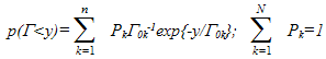
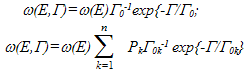
In last equality (15) it is supposed, that there exists n classes of ergodic states in a system; is the probability of that the system will be in k-th a class of ergodic states, is density of distribution of lifetime Γ in this class of ergodic states (generally f_k depends from E). As physical example of such situation (characteristic for metals, glasses) one can mention the potential of many complex systems of a kind, for example, Figure 1. Such situation is considered in[21]. Minima of potential correspond to the metastable phases, disproportionate structures, etc.

Essential object of research of statistical physics recently became complex nonergodic systems: the spin and structural glasses, disorder geteropolimery, the granular media, transport currents, etc.[22]. The basic feature of such systems will be, that their phase space is divided into isolated areas, each of which corresponds to a metastable thermodynamic state, and the number of these areas exponential exceeds full number (quasi)particles[23]. The quasithermodynamical theory of structural transformations of alloy Pd-Ta-H, based on this model, is constructed in[24]. Expression (15) to the description of such systems is applicable.

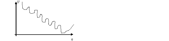
Figure 1. Schematic dependence of thermodynamic potential U on order parameter η in a case potential when the phase space of system is divided into isolated areas, each of which answers a metastable thermodynamic state

We shall assume an obvious kind of distribution , having chosen it as gamma-distribution

(16)

(Γ(α) is gamma-function). We assume, that in k-th metastable area γ=γ_k. We shall choose α_k=γ_k/λ_k; b_k=Γ_0kλ_k/γ_k, λ_k is intensity of energy flow in the system (subsystem), equal in dynamical equilibrium of an output intensity[25]. Then b_kα_k=Γ_0k, ; Γ_0k is equal to average lifetime in k-th a class of metastable states without disturbance, that is, in equilibrium. For average lifetime of the system in dynamical equilibrium state in work[25] by means of stochastic models of storage it is obtained

(17)

where Q_k=exp{-β_kP_kV_k} is the statistical sum of the grand canonical ensemble of the system in k-th a metastable state, β_k=(1/k_BT)_k is return temperature in k-th a metastable state, P_k, V_k, T_k are according to pressure, volume, temperature in k-th a metastable state, V is the full system volume. The value x=γΓ₀=q_at_0a/aR is equal γ(Q-1)/λ, and α=γ/λ= q_at_0a/aR(Q-1). For systems of great volume V, R∼V^1/3, α<<1. Values α can be big for systems of small volume or with small lifetime, with the big currents q_a and great values t_0a, at high temperature (and small β and Q), etc. From (16) follows, that value γ_k from (5)-(7), (10)-(14), (16) which is thermodynamical conjugated to a thermodynamical variable Γ_k in k-th a metastable state, it is proportional to value λ_k, i.e.

(18)

where α_k is parameter of distribution (16). Then from (16) - (17) it is seen that

(19)

For exponential distribution f_k in (16) α_k=1. From (13), (17) at γ=λ we obtain, that <Γ>=Γ₀/Q=(Q-1)λQ. For the big systems, when Q-1 <<1, <Γ>∼1/γ, as in ordinary Boltzmann-Gibbs statistics, ∼1/β=k_BT. At γ≠λ, <Γ>= 1/γ[1+(λ/γ)/(Q-1)]∼1/γ. Substitution (15), (19) in (14) gives

(20)

where u=E/V is specific energy, v_k=V_k/V. Having denoted r₁=P`v`α`/u, α<sub>k</sub>→α`, P_k→P`, v<sub>k</sub>→v`, β₁=(1/k_BT`)_, and replaced summation by integration and entering density of probability f(β₁r₁)=∂P_k/∂(β₁r₁), we obtain from (20):

(21)

For a case of one class ergodic states:

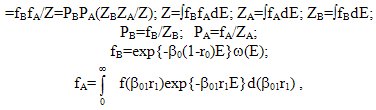
where β is the Lagrange parameter; value β₀=1/k_BT₀ corresponds to average return temperature of full system; k_BT₀ characterizes the conveniently averaged energy; r₀=(P₀/u)α₀ = (P/u)α for full system; lnQ=β₀PV; β=β₀(1-αP/u)=β₀(1-r₀). Substituting this value β in (21) and replacing β₁ by β₀₁=1/k_BT_k=1/k_BT₁(r,t), the fluktuating value of temperature, we get:

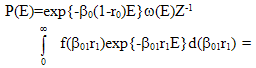
(22)

where f_A and P_A corresponds to the type-A superstatistics from[26]. For f(β₀₁r₁)=δ(β₀₁r₁-β₀r₀) we obtain from (22) the ordinary Boltzmann factor. Equality β₀₁r₁=β₀r₀ it is possible at β₀₁≈β₀, α_kV_kP_k≈αVP. As in[1], we can write down P(E)= exp{-β₀(1-r₀)E}ω(E)Z^-1exp{-β₀r₀E}[1+σ²E²/2+O(σ³E³)]=exp{-β₀E}ω(E)Z^-1[1+(q`-1)(β<sub>0</sub>r<sub>0</sub>)<sup>2</sup>E<sup>2</sup>+g(q`)(β₀r₀)³E³+…], where (q`-1)(β<sub>0</sub>r<sub>0</sub>)<sup>2</sup>=σ<sup>2</sup>, q`=<(β₀r₀)²>/<(β₀r₀)>²; (q`-1)<sup>1/2</sup>=σ/(β<sub>0</sub>r<sub>0</sub>); σ<sup>2</sup>=<(β<sub>01</sub>r<sub>1</sub>)<sup>2</sup>>-(β<sub>0</sub>r<sub>0</sub>)<sup>2</sup>; value β from[1] replace by β<sub>01</sub>r<sub>1</sub>, the fluktuating intensive parameter is equal β<sub>01</sub>r<sub>1</sub> instead of β as in[1]; β<sub>0</sub>r<sub>0</sub>=<β<sub>01</sub>r<sub>1</sub>>= ∫β<sub>01</sub>r<sub>1</sub>f(β<sub>01</sub>r<sub>1</sub>)d(β<sub>01</sub>r<sub>1</sub>), function g(q`) depends on the superstatistics chosen. For f=f_G from (16), (23), q`=q=q<sub>Ts</sub>[2,3]. For others f: q`=q_BC[1]. 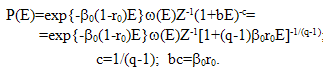For any distribution f(β₀₁r₁) with average β₀r₀=<β₀₁r₁> and variance σ² we can write P(E)∼exp{-β₀(1-r₀)E}01r₁E}>= exp {-β₀E}01r₁-β₀r₀)E}>=exp{-β₀E}[1+σ²E²/2+(-1)^r <(β₀₁r₁-β₀r₀)^r>E^r] similarly[1].

If one performs the replacement of variables β`= β<sub>0</sub>(1-r<sub>0</sub>)+r<sub>1</sub>β<sub>01</sub> and assumes that the situation β<sub>0</sub>=0 is possible, when the bottom limit of integration after replacement of a variable is 0, instead of (22) we shall obtain that P(E)=ω(E)Z<sup>-1</sup>f<sub>1</sub>(β`)exp{-β`E}dβ`, f₁(β`)=f(β<sub>01</sub>r<sub>1</sub>)= f[β`- β₀(1-r₀)], that coincides with superstatistics[1]. But the correlation (22) describes a more general situations and superstatistics forms here a special case (22). The value r₀=α₀(P₀/u). For ideal gas P/u≈0,687. Then 1<α₀<2. Generally, for example, for liquids values u<0 and P/u<0 are possible. This relation and for other, more complex systems is known.

It is possible to mention some examples of physical realization of distribution (22). So, for a case of superdiffusion in[27] at the absence of external force stationary distribution is in Tsallis form, and for a case of presence of constant external force and multiplicate noise in exponential form of distribution is manifested. As in (22), in one phenomenon for one system two kinds of distribution are combined.

Besides the stated scheme there are also other opportunities of realizing the distributions such as (22) and generalizations of the theory of superstatistics. Except for distributions (15)-(16) for density of probability of lifetime in the structural factor ω(E,Γ) (15) one can consider other distributions as well. Since the phase space of complex systems gets intricate fractal structure[28] it is natural to build a distribution on a fractal substrate. As distribution f in (22) it is possible to choose a fractal distributions as in[21] or their generalizations on a case of multifractals, and also other distributions used in[1]. Other various combinations of different distributions in the different purposes are possible as well. The obtained distribution of a kind (22) gives the wide opportunities of the description of various physical situations.

For distribution function f in (22) as gamma-distribution such as (16) (but with variables α_k=c, b_k=b; f(β₁r₁)= Γ^-1(c)b^-c(β₁r₁)^c-1exp{-β₁r₁/b}) expression (22) reduces to the product of Gibbs distribution and Tsallis distribution of a kind

(23)

It is obvious that distribution (22) represents the product of Boltzmann factor with a multiplier superstatistik from which Tsallis distribution as a special case can be obtained (having chosen f in (22) the gamma-distribution of a kind (16)). Comparison of distribution (23) with Boltzmann- Gibbs distribution and with Tsallis distribution shows its intermediate behaviour: tails of distribution fall down not so quickly, as in Gibbs distribution, but also not so slowly, as in Tsallis distribution (Figure 2). If for Gibbs distributions l(u)=exp{-β₀u²/2}/Z (β₀=0,05) tails on borders of the chosen area are equal 1,710^-10, and for Tsallis distribution f(u)=[1+(q-1)β₀u²/2]^1/(1-q)/Z (q=1,46) are equal about 3,710^-4, for distribution (23) k(u)=exp{-β₀(1-r₀)u²/2}Z^-1[1+(q-1)β₀r₀u²/2]^-1/(q-1) (r₀=0,8) they are equal 710^-6 (and equal 1,00410^-9 for p(u) and r₀=0,3006).

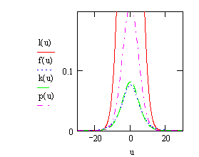
Figure 2. Comparison of distributions (23) k(u)=exp{-β0(1-r0)u2/2}Z-1 (1+(q-1)β0r0u2/2)-1/(q-1) (r0=0,8) and p(u) (r0=0,3006) with Boltzmann-Gibbs distribution l(u)=exp{-β0u2/2}/Z (β0=0,05) and with Tsallis distribution f(u)=[1+(q-1)β0u2/2]1/(1-q)/Z (q=1,46)

The behaviour of distribution (22), (23) essentially depends on values r₀ (α₀). At r₀→ 0 (α₀→ 0, α₀>0) the Gibbs distribution is obtained, and at r₀→1, r₀<1 one gets the Tsallis distribution. At α→ 0 and γ→ 0 (18). As it is marked in the beginning of section 3, it corresponds to transition to Gibbs distributions. Thus and λ→ 0, but also α=γ/λ→ 0 also it is performed correlation (17). The value γ describes entropy fluxes and entropy production in the system; the value λ describes intensity of an input in system (and an output from it).

Distribution of a kind (23) was used by us for the description self-organized criticality (SOC)[29]. In work[30] formation of a stationary single avalanche and fluktuated formation of an avalanche in view of additive noise for a component of speed and an inclination of sand are considered. Thus distribution of the order parameter acquires a power-like form with an integer parameter. But generally this parameter should be fractional, therefore in[30] generalization of system of Lorentz is performed allowing to account for the behaviour of ensemble of avalanches. Stochastic systems for not additive ensemble of avalanches are used also. We have performed calculation on distribution (23) with effective energy

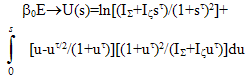
from[30] for a case fluktuated formations of avalanches with an integer exponent of distribution of parameter of the order τ=2 also have compared behaviour of stationary distribution to the results received in[30] (Figure [30]) for a case τ=1,5 in distribution exp{-U(s)}/Z. The results are shown in Figure 3. Calculation was carried out for the same values of parameters noise intensivity of energy I∑ and complexity Iζ which are used in[30]. Concurrence of the results, similar behaviour of distributions is evidenced. Parameters q, r0 only weakly influence behaviour of distribution. We shall note, that using the pure Tsallis distribution leads to another behaviour of stationary distribution (in particular, does not show indicated in[30] distinctions between distributions with I∑=1; Iζ=5 and I∑=0,5; Iζ=30).

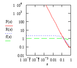
Figure 3. Function of distribution (23) in the description self-organized criticality (SOC) at τ=2, q-1=4/11, r0=0,1; P(s) (R(s), f(s))=[1 + 0,1(q-1) U(s)]-1/cexp{-0,9U(s)}; U(s)=ln[(I∑+Iζsτ)/(1+sτ)2]+ [u-uτ/2/(1+uτ)][(1+uτ)2/(I∑+Iζuτ)]du; P(s): I∑=0; Iζ=50; R(s): I∑=0,5; Iζ=30; f(s): I∑=1; Iζ=5.

Figure 4. Energy spectrum of primary cosmic rays (in units of m-3s-1sr-1 GeV-1) as listed in[31]. The line p(E) is the prediction by p(E)=CE2(1+(q-1)E)-1/(q-1) with q=1,215, -1=kB=107 MeV, C=510- the above units[31]. The function f(E)=CE2exp{- (1-r0)E}(1+(q-1) r0E)-1/(q-1) obtained on (23) with r0=1-10-14. Functions g(E), k(E), r(E), s(E), e(E) too are obtained on expression (23) with r0=1-10-13 , r0=1-10-12 , r0=1-10-11 , r0=1-10-10 , r0=1-10-9 accordingly

Comparison with the results received in works[31,32] for a spectrum of the cosmic ray was carried out as well. By means of distribution of a kind p(E)=CE²(1+(q-1)E)^-1/(q-1) (C is a constant representing the total flux rate; the Tsallis distribution is multiplied with E², taking into account the available phase space volume) at q=1,215, ^-1=107 MeV, C=510^-[31] the measured flux rate of cosmic ray particles with a given energy is well fitted. If we use for these purposes the distribution (23) multiplied with CE² there is an additional parameter r₀ (Figure 4). At values r₀ close to 1 we get coincidence to results of[31]. At r₀=1-10^-14 the coincidence to results[31] is exact. At r₀=1-10^-13 sharper bend is obtained at ankle energy ∼ 10¹⁹ eV; the plot for flux rate comes nearer to curve for parameters q=11/9, C=10^-14 from[31] as well. Decreasing r₀ we get the dependence, characteristic for Boltzmann-Gibbs distribution, resulted on Figure [32]. At values r₀≈1 it is possible to explain conformity of experimental data in small volume of system both high energy and temperatures. Comparison of calculations was carried out also by means of expression (23) with estimations of distributions for the motion of point defects in thermal convection patterns in an inclined fluid layer[26,33] which also has shown conformity with the results received in[26,33].

5. Conclusions

The results of Sections 2-4 were investigated in[4-5]. From the distribution (5) containing lifetime of statistical system (time before degeneration of system) are obtained the superstatistics, entered in[1] in many respects is formal (though in[1] the dynamic bases is lead). In the present work obvious expression for β`=β<sub>0</sub>(1-r<sub>0</sub>)+r<sub>1</sub>β<sub>01</sub> is obtained, the physical sense of distributions f<sub>1</sub>(β`) and f(α_kβ_kP_k/u_k) is elucidated (besides distribution of return temperature), - as density of distribution of probability of destruction in the certain time interval, on k-th stages. It is possible for this reason gamma-distributions f(x)=λαxα^-1 exp{-λx}/(α) with a parameter α=r/2 (is more true, χ² distributions with r degrees of freedom which corresponds to gamma-distribution at λ=1/2-c; in[1] value r is interpreted as number of degrees of freedom giving the contribution in fluktuating value β) precisely describe Tsallis statistics, - they correspond to distribution of lifetime with r stages.

Other variant of the obtained expressions forms at lnQ=βPV instead of β₀PV as it was supposed after expression (21). Then β₀=β(1+r₀), β=β₀/(1+r₀), and correlations (22), (23) become the form P(E)=exp{-β₀E/(1+r₀)}ω(E)Z^-1f(β₀₁r₁/(1+r₀))exp{-β₀₁r₁E/(1+r₀)} d(β₀₁r₁/(1+r₀)); P(E)=exp{-β₀E/(1+r₀)}ω(E)Z^-1[1+(q-1)β₀r₀E/(1+r₀)]^-1/(q-1). At r₀→0, α→0, these distributions pass in Gibbs distribution, as in (22), (23). But in Tsallis distribution they pass at r₀→∞, α→∞, γ→∞ as against (22), (23) where it occurs at r₀=αP/u=1, α=u/P=γ/λ. Possible relation of values β_q=β/=β/[1-(q-1)S_q][34] with β₀=β/(1-r₀) or β(1+r₀) depends on a choice of β as well. Thus it is possible to find a relation between α and q. In[34] one more interesting question on a form of the differential equations for y(x)=P(E) is considered. For distribution (23) this equation looks like dP(E)/dE=-β₀(1-r₀)P(E)-β₀r₀P(E)/[1+(q-1)β₀r₀E]. It is possible to lead analogies to the equations which have been written down in[34].

The Gibbs distribution does not describe the dissipative processes that develop in the system. Superstatistics describe systems by constanly putting energy into the system which is dissipated. The value α=γ/λ is connected with dissipative processes in the system (through γ). She defines a correlation between Gibbs and superstatistics multipliers in distribution (22).

It is possible not to pass to integrated relations, as in (22), having limited to summation (so, as discrete analogue of gamma-distribution negative binomial distribution serves). The discrete description in many cases, for example, for bistability potential, appears more precisely continuous. The found conformity between superstatics and the nonequilibrium distribution containing lifetime, should appear useful to both cases. For example, many results established for superstatistics and nonextensive statistical mechanics, are transferred to the description of complex systems by means of the distribution containing lifetime. Since thermodynamics with lifetime[4, 5] is more general, than the theory of superstatistiks also it has more opportunities. Interesting is establishing the relation to a method of the nonequilibrium statistical operator of Zubarev[11] generalizing Gibbs distributions which as it was marked, it is possible to compare to the distributions containing lifetime, and nonextensive statistical mechanics[2-3], in which entropy is represented by means of the measures which are distinct from Boltzmann and Gibbs. Probably, they stand close to the concept of lifetime, in the latent kind present in both theories. The relation γ=αλ (18) is of interest also. The value γ thermodynamical conjugated to random lifetime is expressed through entropy production and currents[12], i.e. through communication of system with an environment.

It is shown, that the behaviour of the obtained distribution (22)-(23) interpolates between behaviour of Gibbs and Tsallis distributions. Application of this distribution to the phenomenon of the self-organized criticality (and other examples) shows his efficiency. The obtained distribution contains the new parameter related to a thermodynamic state of the system, and also with distribution of a lifetime of a metastable states and interaction of this states with an environment. Changing this parameter it is possible to pass to both Gibbs and Tsallis distributions.

References

[1]  C. Beck and E.G.D. Cohen, Physica A 322A, 267 (2003), (cond-mat/0205097).
[2]  C. Tsallis, J.Stat.Phys. 52, 479 (1988).
[3]  http://tsallis.cat.cbpf.br/biblio.htm .
[4]  V.V. Ryazanov, European Physical Journal B 72, 629 (2009).
[5]  V.V. Ryazanov, S.G. Shpyrko, Condensed Matter Physics 9, 71 (2006).
[6]  M.A. Leontovich, Introduction to Thermodynamics. Statistical Physics (in Russian) (Nauka, Moscow, 1985).
[7]  W. Feller, An Introduction to Probability Theory and its Applications, vol.2 (J.Wiley, New York, 1971).
[8]  Е.Е. Kovalev, А.I. Vichrov, V.G. Semenov, Atomnaya energiya 83, 291 (1997).
[9]  P. Hanggi, P. Talkner, M. Borkovec, Rev.Modern Phys. 62, 51 (1990).
[10]  R.L. Stratonovich, Nonlinear Nonequilibrium Thermodynamics (Springer, Heidelberg, 1992).
[11]  D.N. Zubarev, Nonequilibrium Statistical Thermodynamics (Consultants Bureau, New York, 1974).
[12]  V.V. Ryazanov, Fortschritte der Phusik/Progress of Physics 49, 8852001 (2001).
[13]  R. Dewar, J.Phys.A: Math. Gen. 36, 631 (2003).
[14]  Yu.L. Klimontovich, Statistical Theory of Open Systems (Kluwer Acad. Publ., Dordrecht, 1995).
[15]  E.T. Jaynes, Phys.Rev 106, 620; 108, 71 (1957).
[16]  V.S. Korolyuk, A.F. Turbin, Mathematical Foundations of the State Lumping of Large Systems (Kluwer Acad.Publ., Dordrecht, Boston/London, 1993).
[17]  D. Jou, J. Casas-Vazquez, G. Lebon, Extended Irreversible Thermodynamics (Springer, Berlin, 1996).
[18]  P. Gaspard, G. Nicolis, Phys.Rev.Lett. 65 (14), 1693 (1990).
[19]  J.R. Dorfman, P. Gaspard, Phys.Rev.E 51, 28 (1995).
[20]  P. Gaspard, J.R. Dorfman, Phys.Rev.E 52, 3525 (1995).
[21]  A.I. Olemskoi, Physics-Uspekhi 163, 1 (1993).
[22]  J.P. Bouchaud, L.F. Gudliandolo, J. Kurchan, Spin Glasses and Random Fields. Ed. A.P.Young (World Scientific, Singapore, 1998).
[23]  S.F. Edwards, Granular Matter: an Interdisciplinary Approach. Ed. A. Metha (Springer-Verlag, New York, 1994).
[24]  V.M. Avdyukhina, A.A. Katsnelson, A.I. Olemskoi, D.A. Olemskoi, G.P. Revkevich, Physics of the solid state 44, 979 (2002).
[25]  V.V. Ryazanov, Ukrainian Journal of Physics (Kiev,Ukraine; in Russian) 38, 15 (1993).
[26]  C. Beck, cond-mat/0303288.
[27]  A.I. Olemskoi, D.A.Kharchenko, Journal of Physical Studies 6, 53 (2002).
[28]  A.I. Olemskoi, Physics-Uspekhi 168, 287 (1998).
[29]  P. Bak, C. Tang, K. Wiesenfeld, Phys Rev. Lett. 59, 381 (1987).
[30]  A.I. Olemskoi, D.A. Kharchenko, Journal of Physical Studies 7, 1 (2003).
[31]  C. Beck, cond-mat/0301354.
[32]  C. Tsallis, J.C. Anjos, E.P. Borges, astro-ph/0203258.
[33]  K.E. Daniels, C. Beck, E. Bodenschatz, cond-mat/0302623.
[34]  C. Tsallis, cond-mat/0403012v1.