G. M. Moatimid , M.H.M. Moussa , Rehab M. El-Shiekh , A. A. El-Satar
Department of Mathematics, Faculty of Education, Ain Shams University, Roxy, Hiliopolis, Cairo, Egypt
Correspondence to: A. A. El-Satar , Department of Mathematics, Faculty of Education, Ain Shams University, Roxy, Hiliopolis, Cairo, Egypt.
| Email: |  |
Copyright © 2012 Scientific & Academic Publishing. All Rights Reserved.
Abstract
In this paper, Lie-Group method is applied to the b-family equations which includes two important nonlinear partial differential equations Camassa--Holm (CH) equation and the Degasperis--Procesi (DP) equation. The complete Lie algebra of infinitesimal symmetries is established. Three nonequivalent sub-algebras of the complete Lie algebra are used to investigate similarity solutions and similarity reductions in the form of nonlinear ordinary equations (ODEs) for the b-family equations. The generalized He's Exp-Function method is used to drive exact solutions for the reduced nonlinear ODEs, some figures are given to show the properties of the solutions.
Keywords:
Similarity Reductions, Lie-Group Method, Exact Solution
1. Introduction
In this paper we consider the following b-family of equations[1]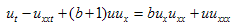 | (1.1) |
where b is a dimensionless constant. The quadratic terms in Eq. (1) represent the competition, or balance, in fluid convection between nonlinear transport and amplification due to b-dimensional stretching[2-3]. On the other hand, in a recent study of soliton equations, it was found that for any b≠-1, Eq. (1) was included in the family of shallow water equations at quadratic order accuracy that are asymptotically equivalent under Kodama transformations[4].Degasperis and Procesi[5] showed that the family of equations (1) cannot be integrable unless b=2 or b=3 by using the method of asymptotic integrability. The previous two values of b are corresponding to two important equations the Camassa--Holm (CH) equation and the Degasperis-- Procesi (DP) equation respectively. The CH and the DP equations are bi-Hamiltonian and have an associated isospectral problem, therefore they are both formally integrable[6-9]. Moreover, both equations admit peaked solitary wave solutions and present similarities although they are truly different[10-13].
2. Solution of the Problem
Firstly, we shall derive the similarity solutions using the Lie group method[14] under which Eq. (1.1) is invariant in the following steps:1- Lie point symmetries | (2.1) |
With associated infinitesimal form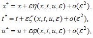 | (2.2) |
2- If we set | (2.3) |
Then the invariance condition | (2.4) |
where  is given by
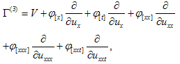 | (2.5) |
where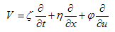 | (2.6) |
The components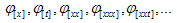 | (2.7) |
can be determined from the following expressions: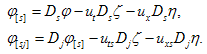 | (2.8) |
Eq. (2.4) gives the following system of linear partial differential equations: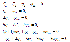 | (2.9) |
3- The general solution of Eqs. (2.9) provides following forms for the infinitesimal element ζ,η and φ: | (2.10) |
where c1,c2 and c3are arbitrary constant.4- In order to study the group theoretic structure, the vector field operator V is written as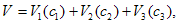 | (2.11) |
where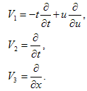 | (2.12) |
It is easy to verify the vector fields are closed under the Lie bracket as follows: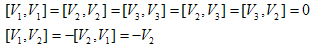 Furthermore, we can compute the adjoint representations of the vector fields
 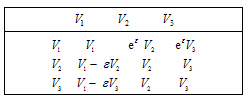 From the previous adjoint representations we have the following three non-equivalent possibilities of sub-algebras of the Lie algebra (I) V1+V3.(II) V2+V3.(III) V1.Now we could determine the similarity variables and similarity reduction corresponding each vector field using the auxiliary equation
 | (2.13) |
3. Similarity Reduction and Exact Solutions
In this section, the primary focus is on the reductions association with the vector fields (I-III) and attempt to some exact solutions:Vector field V1+V3For this vector field, on using the characterstic Eq. (2.13), the similarity variable and the form of similarity solution is as follows: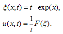 | (3.1) |
On using these in Eq. (1.1), the reduced ODE is given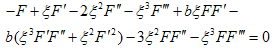 | (3.2) |
where prime (′) denotes the differentiation with respect to the variable ξ. On transforming the independent variable by the relation ξ=exp(τ) Eq. (3.2) becomes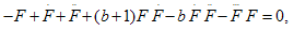 | (3.3) |
where dot denotes the defferentiation with respect to variable τ. In view of the generalized He's Exp-Function method[15], we assume that the solution of Eq. (3.3) can be expressed in the form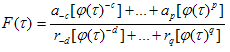 | (3.4) |
where c, d, p and q are positive integers which are unknown to be further determined, an and rm are unknown constants. In addition, φ(τ) satisfies Riccati equation, | (3.5) |
In order to determine values of c and p, we balance the linear term of the highest order in Eq. (3.3), we have | (3.6) |
 | (3.7) |
where ai and ri are determined coefficients only for simplicity. From balancing the lowest order and highest order of φ (3.6) and (3.7), we obtain | (3.8) |
which leads to the limit | (3.9) |
and | (3.10) |
which leads to the limit | (3.11) |
For simplicity, we set p = c = 1, the trial function, Eq. (3.4), becomes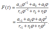 | (3.12) |
Substituting Eq. (3.12) into Eq. (3.3), equating to zero the coefficients of all powers of φ(τ) yields a set of algebraic equations for a₀, r₀, a0, r1, a-1 and r-1 . Solving the system of algebraic equations with the aid of Maple, where A= , B=0, C=
 in Eq.(2.18), we obtain the following results:
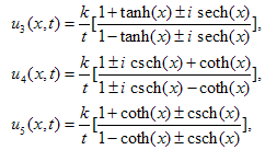
 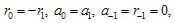 b is arbitrarySubstituting the results of case I into (3.12), the solutions of Eq.(1.1) can be written as:
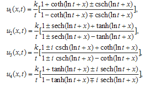 | (3.13) |
where .Vector field V2+V3For this generator the associated similarity variable and similarity solution are given by:
 | (3.14) |
On using these in Eq. (1.1), the reduced ODE is given by  | (3.15) |
Be using the ansatz (3.14), the solution of Eq. (1.1) can be writen as: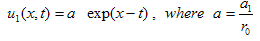
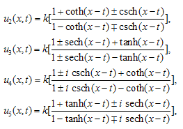 | (3.16) |
where  Vector field V1The generator (III) in the optimal system defines the similarity variable and similarity solution as follows:
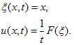 | (3.17) |
On using these in Eq. (1.1), the reduced ODE is given by | (3.18) |
Using the ansatz (3.14), we have the following solutions: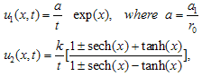
 | (3.19) |
where 
4. Conclusions
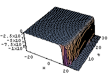
In summary, we have utilized this method to construct new exact solutions for b-family equations. In solutions (3.13) and (3.19) there is singularity at t=0, so we put t≻0 in figures. All solutions have been obtained in this paper for the b-family equations are also solutions for the CH and DP equations because those solutions were not restricted with any value of b.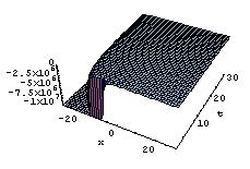 | Figure 1. solution of u1 (x,t) in (26), where k=1 |
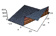 | Figure 2. solution u1 (x,t) in (29), where k=1 |
 | Figure 3. solution u1 (x,t) in (29), where k=1 |
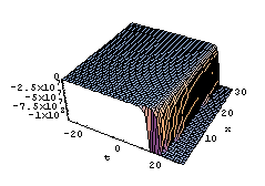
 | Figure 4. solution u1 (x,t) in (32), where k=1 |
References
| [1] | A. Degasperis, D.D. Holm, A.N.W. Hone, Theoret. and Math. Phys. 133 (2002) 170-183. |
| [2] | A. Degasperis, D.D. Holm, A.N.W. Hone, II (Gallipoli, 2002), 37.43, World Sci. Publishing, River Edge, NJ, 2003. |
| [3] | H.R. Dullin, G.A. Gottwald, D.D. Holm, Phys. Rev. Lett. 87 (2002) 4501. 4504. |
| [4] | Degasperis A and Procesi M, Rome, December 1998, World Scienti.c, River Edge, NJ, 1999, 23-37. |
| [5] | Camassa R and Holm D, Phys. Rev. Lett. 71 (1993), 1661-1664. |
| [6] | Constantin A, Proc. R. Soc. London Ser. A - Math. Phys. Eng. Sci., 457 (2001), 953.970. |
| [7] | Constantin A and McKean H P, Comm. Pure Appl. Math. 52 (1999), 949.982. |
| [8] | Lenells J, J. Non-linear Math. Phys. 9 (2002), 389.393. |
| [9] | Fuchssteiner B and Fokas A S, Phys. D 4 (1981), 47.66. |
| [10] | Constantin A and Molinet L, Comm. Math. Phys. 211 (2000), 45.61. |
| [11] | Constantin A and Strauss W, Comm. Pure Appl. Math. 53 (2000), 603-610. |
| [12] | Octavian G Mustafa. Non linear Math. Phys.12 (1) (2005)10-14. |
| [13] | P.J. Olver, New York (1986). |
| [14] | A. El-Halim Ebaid, znaturforsch, 2009 |
 Abstract
 Reference
 Full-Text PDF
 Full-Text HTML