M. Gherda 1, M. Boushaba 2
1Department of Mathematics, Faculty of sciences, University of Jijel, Algeria
2Laboratory of mathematical modeling and simulation, University of Constantine Route d'Aïn-El-Bey Constantine, Algeria
Correspondence to: M. Boushaba , Laboratory of mathematical modeling and simulation, University of Constantine Route d'Aïn-El-Bey Constantine, Algeria.
| Email: |  |
Copyright © 2012 Scientific & Academic Publishing. All Rights Reserved.
Abstract
An (n-1)-out-of-n: G system is a system that consists of n components and works if and only if (n-1) components among the n work simultaneously. The system and each of its components can in only one of two states: working or failed. When a component fails it is put under repair and the other components stay in the working state with adjusted rates of failure. After repair, a component works as new and its actual lifetime is the same as initially. If the failed component is repaired before another component fails, the (n-1) components recover their initial lifetime. The lifetime and time of repair are independent. In this paper, we propose a technique to calculate the mean time of repair, the probability of various states of our system and its availability by using the theory of distribution.
Keywords:
G System, System Availability, Reparable System, Failure Rates, Distribution Theory
Cite this paper:
M. Gherda , M. Boushaba , "Analysis of a Repairable (n-1)-out-of-n: G System with Failure and Repair Times Arbitrarily Distributed", American Journal of Mathematics and Statistics, Vol. 1 No. 1, 2011, pp. 1-7. doi: 10.5923/j.ajms.20110101.01.
1. Introduction
The k-out-of-n system structure is a very popular type of redundant fault-tolerant systems. It finds wide applications in both industrial and military systems. These systems include the multidisplay system in cockpits, the multiengine system in an airplane, and the multipurpose system in a hydrau-lic control system. In a communications system with three transmitters, the average message load may be such that at least two transmitters must be operational at all times or critical messages may be lost. The transmission subsystem functions as a 2-out-of-3: G system. Systems with spares may also be represented by the k-out-of-n system model. In the case of an automobile with four tires, for example, usually one additional spare tire is carried on the vehicle. Thus, the vehicle can be driven as long as at least 4-out-of-5 tires are in good condition. In this paper, we consider the repairable case where k=n-1, i.e. a repairable (n-1)-out-of-n: G system which works if and only if at least (n-1) components among the n work simultaneously. Few papers analyze this kind of systems, Gaver[1] and Jack[2] consider a 2-unit parallel system, Gherda & Boushaba[3] analyze a 2-out-of-3 system when the distributions of the time of failure and the time of repair are general. In this work, we generalize the result of Gherda & Boushaba[3]: We suppose that all components and the system have either one of two states: a "working" state or a "failed" state. whena component fails it is put under repair and the other components stay in the "working" state with adjusted rates of failure. After repair, the component works as new and its actual lifetime is the same as initially. If the failed component is repaired before another component fails, the (n-1) components recover their initial lifetime. The lifetime and time of repair are independent. In this paper, we propose a technique to calculate the mean time of failure, the probability of various states of our system and its availability by using the theory of distribution. Finally, we give some numerical examples.
2. Notation
 : component of the system, i=1,2,...,n
 : the state of system, s=0, 1, 2.We say that the system is in the state
  at time t if there are exactly s failed components at time t.
 : rate of failure of component
  when all components j, (i≠j) are working.
 : rate of failure of component
  when component j,(i≠j) is "failed".
 : time of repair of component
  .
. : the density of the probability of event: " only the component
  is fails at time t and it is under repair since a time x"
 : the density of probability of event : "Two components
  and
and  are "failed" and components
  are in the "working" state at time t since time x; i∈{1,...,n}/{j; k}.
 : Probability of the event: "No component is "failed" at time t"
 : The Laplace transform of the distribution of TA: The availability of the system
 : the distribution function of
  and
and 
 : hazard rate function
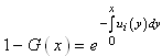 and.
and.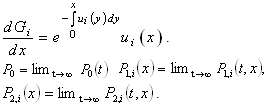
 : the Laplace transform of
  and
and 
 : the inverse Laplace transform of
  *: Convolution product
3. Model
Let N (t) and X (t) be two stochastic process with continuous time such that N (t) = s.If the system is in the state  and X (t) = x if the component which failed at time t is under repair since date x:Consider the event N (t + dt) = 0; it can be obtained in (n + 1) different ways:- At time t, N (t) = 0 and during the interval of time [t; t + dt] there are no failures, the probability of this event is
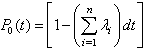 Or at time t, N (t) = 1 and during the interval of time [t; t + dt]; the failed component C is repaired, the probability of this event is
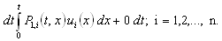 Then the probability of this event is
 when
when  we obtain
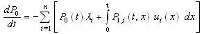 | (1) |
Consider the event N (t + dt) = 1; it can be obtained in 2n different ways :- N (t + dt) = 1 and X (t + dt) = x + dt: if N (t) = 1, X (t) = and the repair of the failed component is not finished at time t + dt: the probability of this event noted by
 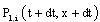 is given by:
 otherwisewhen
  we obtain:
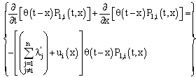 | (2) |
where  is the indicator function.- Or N (t + dt) = 1 and X (t + dt) = dt: if N (t) = 0 and a failure occurs during the interval of time [t; t + dt]: This case is given by the initial conditions:
  Our system can be represented by the figure1.
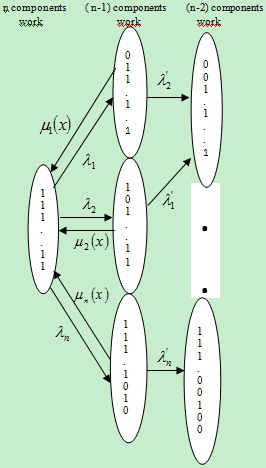 | Figure 1. |
4. Calculation of the State Probabilities of a System
4.1. Calculation of  and
and 
Let  and
and  be the Laplace transform of
  and
and  respectively. Because the indicator function
  is a regular distribution, we can use the derivation of (2) in the sense of distribution:
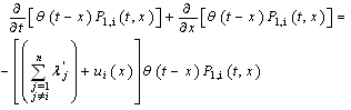 By taking the Laplace transform of the two members of this last equality we obtain
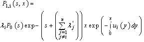 | (3) |
Now, taking the Laplace transform of the two members of the equality (1):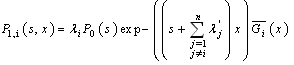 | (4) |
we note that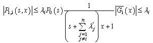 by applying a proposition in[4] page 252 to
 , which verifies this majoration, we obtain
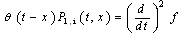 where
where  is the inverse transform of
  We note that
  is the Laplace transform of the convolution product. By using (4 ):
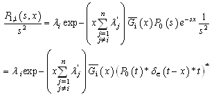 where
where  is the Dirac function. The inverse Laplace transform of
  is given by:
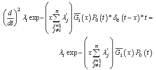 | (5) |
Now, we obtain: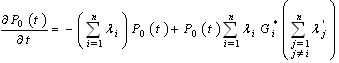 By taking the Laplace transform of the two members of this equality we obtain:
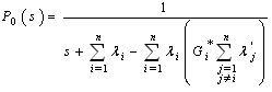 by using the inverse Laplace transformed, we obtain:
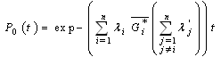 and
and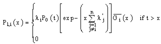 otherwiseWith conditions
 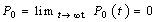 and
and 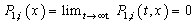
4.2. Calculation of 
The event N(t + dt) = 2 can be obtained in two ways:1. N(t) = 1, X(x+dt) = dt; X(t) =  and during the interval of time [t; t + dt], one component among the working components fails and the repair of the failed component is not finished. This event has the probability:
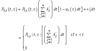 otherwise2. Or N(t) = 2 , X(x + dt) = dt, and any repair are finished and no failure occurs during the interval of time [t; t + dt] :This event has the probability:
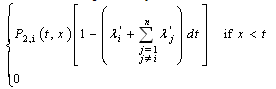 otherwiseSo
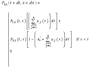 when
when  we obtain:
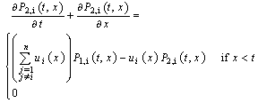 Otherwise, by using the Laplace transform and the initial condition Pi (t; t) = 0, we obtain:
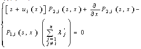 | (6) |
One solution of this equation is given by: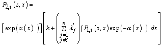 where
where  is a primitive of
  and k a constant.Now by using the convolution product, the solution of (6) is given by
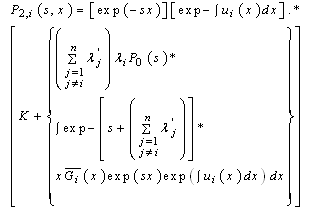 finally, we obtain :
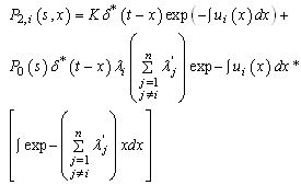 by using the inverse Laplace transform and the initial condition Pi (t; t) = 0 (K = 0), we obtain
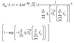 and
and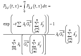
5. Characteristics of the System
5.1. Mean Time of Failure
Let  be the Laplace transform of
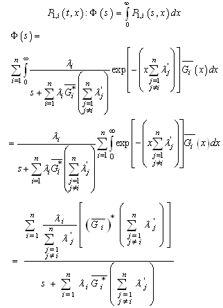 Finally
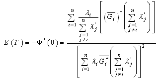
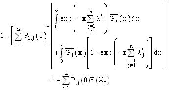
5.2. Availability of the System
Let  the availability of the system. Then
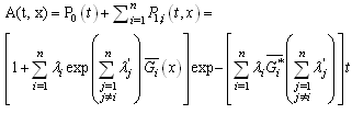
5.3. Case of n Non Identical Components
In the stability case, we obtain the following equations for the system: This system becomes:
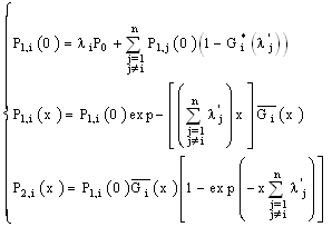 by using this hypothesis:
 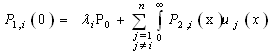 (conditions at the limits), we obtain
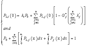 So
So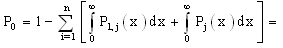
 we can write the solution in the following form:
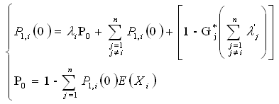 finally, we derive:
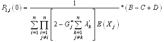 Where
Where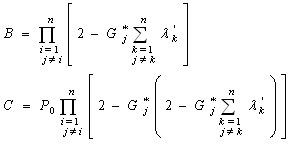 and
and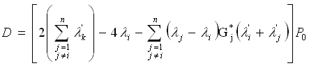
5.4. Case of N Identical Components
In the stability case ( ), we obtain the following equations for the system:
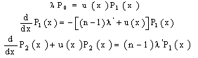 by using the initial conditions and conditions at the limits :
 and
and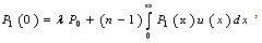 ,we obtain
 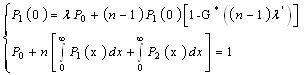 By the same argument as in the non identical case, we derive
 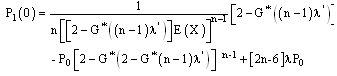 Remark 1: when n=3, we obtain the result given in page [3]
6. Numerical Examples
Consider the case where n=2 and the stability case  . When the components are non identical, the equations of the system are:
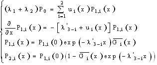 By combining these equations, we obtain:
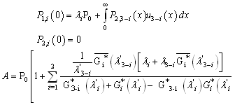 where
where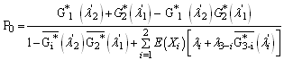 In the identical case, we have
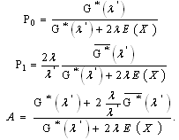 In the following, we will give some numerical examples when we consider the cases:-X is constant,
 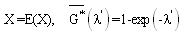 -X follows the exponential law
 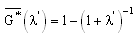 - X follows the law
 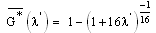 We note
  if
if  and
and  , the values of E(X) for different values of m and different laws of X are given in Tables 1 and 2, respectively:
Table 1. The values of E(X) for different values of m and different laws of X.(
 ) ) |
|

| X=ct |

|

| | 0.5 | 13.2 | 33.7 | 64 | | 1 | 8.5 | 9.77 | 23 | | 1.5 | 4.1 | 5 | 13 | | 2 | 2.5 | 3 | 9 |
|
|
| Table 2. The values of E(X) for different values of m and different laws of X.() |
|

| X=ct |

|

| | 0.5 | 8.5 | 9.77 | 23 | | 1 | 2.5 | 3.1 | 9 | | 1.5 | 1.3 | 1.7 | 5.3 | | 2 | 0.6 | 3 | 3.7 |
|
|
The values of the probability states and the availability, for various laws of X, are given in the Tables 3, 4 and 5.| Table 3. The values of probability y states and availability for X constant |
|

|

| P0 | P1 | P2 | A | | 0.5 | 0.375 | 0.52 | 0.217 | 0.02 | 0.96 | | 1 | 0.375 | 0.48 | 0.216 | 0.04 | 0.91 | | 1.5 | 0.375 | 0.43 | 0.215 | 0.07 | 0.86 | | 2 | 0.375 | 0.38 | 0.214 | 0.09 | 0.82 | | 0.5 | 0.75 | 0.31 | 0.28 | 0.06 | 0.88 | | 1 | 0.75 | 0.24 | 0.26 | 0.11 | 0.77 | | 1.5 | 0.75 | 0.18 | 0.24 | 0.16 | 0.67 | | 2 | 0.75 | 0.13 | 0.22 | 0.21 | 0.58 |
|
|
Table 4. The values of probability y states and availability for
 |
|

|

| P0 | P1 | P2 | A | | 0.5 | 0.375 | 0.53 | 0.2 | 0.04 | 0.92 | | 1 | 0.375 | 0.49 | 0.18 | 0.07 | 0.86 | | 1.5 | 0.375 | 0.46 | 0.17 | 0.10 | 0.80 | | 2 | 0.375 | 0.43 | 0.16 | 0.12 | 0.75 | | 0.5 | 0.750 | 0.49 | 0.21 | 0.04 | 0.92 | | 1 | 0.750 | 0.43 | 0.19 | 0.09 | 0.81 | | 1.5 | 0.750 | 0.38 | 0.16 | 0.14 | 0.72 | | 2 | 0.750 | 0.35 | 0.14 | 0.17 | 0.64 |
|
|
7. Conclusions
The work presented here is a study of a (n-1)-out-of-n: G repairable system whose components are independent and not identical. The duration of component failure and that of the repairs are random variables following exponential laws and arbitrary laws respectively. The novelty in this contribution is the use of the following, very realistic hypothesis: when a component fails, the failure rates of all other components change; naturally, when that component is repaired, these same components recover their initial failure rates. To the authors’ knowledge, previous works did not tackle this case from the same angle as this study. The authors believe that differentiation of distributions is the technique best suited for the calculation of the availability and of the other characteristics of this kind of systems. Additionally, the choice of the technique to use is believed to be judicious and has never been used before in this kind of situations. More generally, the case k-out-of-n systems remains an open problem that deserves more exploration.Table 5. The values of probability y states and availability for
 |
|

|

| P0 | P1 | P2 | A | | 0.5 | 0.375 | 0.355 | 0.064 | 0.26 | 0.48 | | 1 | 0.375 | 0.352 | 0.045 | 0.28 | 0.44 | | 1.5 | 0.375 | 0.350 | 0.036 | 0.29 | 0.42 | | 2 | 0.375 | 0.340 | 0.030 | 0.30 | 0.40 | | 0.5 | 0.75 | 0.270 | 0.070 | 0.30 | 0.41 | | 1 | 0.75 | 0.265 | 0.046 | 0.32 | 0.36 | | 1.5 | 0.75 | 0.263 | 0.350 | 0.33 | 0.33 | | 2 | 0.75 | 0.260 | 0.030 | 0.34 | 0.31 |
|
|
ACKNOWLEDGEMENTS
The authors are grateful for Professor Fabrizio Ruggeri from IMATI (Italy) for the valuable suggestions and comments which have considerably improved the presentation of the paper.We acknowledge, with thanks, the constructive comments made by the referees which helped to enhance the quality of this paper.
References
| [1] | D. P. Gaver, Time to failure of paralled systems with repair, IEEE transaction on reliability, vol R-11, 1962 |
| [2] | N. Jack, Analysis of a repairable 2-unit parallel redundant system with repair, IEEE transaction on reliability, vol R-35, 1986 |
| [3] | M. Gherda and M. Boushaba, Analysis of a repairable 2-out-of-3 system with failure and repais times arbitrarily distributed, procceding of 13th ISSAT international conference, Seattle, Washington, USA, august 2-4 2007, eds: T. Nakagara, H. Pham and S. Yamada, pp 196-200 |
| [4] | L. Shwartz, Méthodes mathématiques pour les sciences physiques, 1966, eds Herman Paris |
| [5] | K. N. Francis Leung, Y. L. Zhang, K. K. Lai, Analysis for a two-dissimilar-component cold standby repairable system with repair priority, Reliability Engineering and system safety, vol. 96 issue 11, November 2011, pp 1542- 1551 |
| [6] | Y. L. Zhang, G. J. Wang, A geometric process repair model for a repairable cold standby system with priority in use and repair, Reliability Engineering and system safety, vol. 94 issue 11, No-vember 2009, pp 1782-178 |
 Abstract
 Reference
 Full-Text PDF
 Full-Text HTML