Akifa Akther , Rafiqul Islam
Department of Population Science and Human, Resource Development, University of Rajshahi, Rajshahi , 6205, Bangladesh
Correspondence to: Rafiqul Islam , Department of Population Science and Human, Resource Development, University of Rajshahi, Rajshahi , 6205, Bangladesh.
| Email: |  |
Copyright © 2012 Scientific & Academic Publishing. All Rights Reserved.
Abstract
The aim of this research is to study age at menarche of school going girls in . For this purpose, the data is acquired from of the classes of five, six, seven and eight during1st June. In this study, it is to investigate the pattern of age at menarche of total respondents and the pattern of height, weight and body mass index by the age of the respondents in accordance with menarche and non-menarche. The age range of the respondents was between 10 to 14 years. Chi-square test and logistic regression analysis are employed in this paper. This study also displays the association of age at menarche with socio-demographic variables of respondents. It is realized from the association that early menarche for school going girl’s height, weight, father income, body mass index, time spent by watching television and father educational qualification were highly significant but mother educational qualification, mother occupation, father occupation, number of siblings, order of birth, time spent by playing and mother time spent were insignificant. In logistic analysis, it was found that only height, weight and time spent by watching TV were significant which have positive effects on age at menarche.
Keywords:
Age at menarche, Chi-square test, Logistic regression analysis, Model validation technique
1. Introduction
Menarche is a part of complex process of physical and emotional development of a girl. The cyclical release of blood, mucous in certain other substances per vagina from uterus in the reproductive span, that is, ages of 15 to 49 years of life of the female at standard period of about 28 days is called menstruation. The cyclic production of humorous that culminates in the release of a mature egg, that is, ovum, is called the menstrual cycle and the first menstrual cycle is called menarche. Menarche is the first menstrual period, or first menstrual bleeding of the female of human beings. From both social and medical perspectives menarche is influenced by both genetic and environmental factors, especially nutritional status. The average age of menarche has declined over the last century but the magnitude of the decline and the factors responsible remain subjects of contention. Age at menarche is an important indicator of future diseases. Early onset of menarche is a well-established risk factor for breast cancer[1]. It might also increase the risk of heart disease[2]. Late menarche may, however, be positively associated with the risk of developing Alzheimer’s disease [3]. Age at menarche may also affect reproductive function. Early menarche may be a marker for reproductive fitness or, at least, a marker for the onset of childbearing years[4]. In consequence, early menarche is the main cause of high fertility as well as high mortality. Changes in mean age at menarche over time may underlie the changing patterns of these diseases. On the other hand, not every girl follows the typical pattern, and some girls ovulate before the first menstruation. Although unlikely, it is possible for a girl who has engaged in sexual intercourse shortly before her menarche to conceive and become pregnant, which would delay her menarche until after the birth. This goes against the widely held assumption that a woman cannot become pregnant until after menarche.Since the 18th century secular trends in age at menarche have been described. Results from Western countries are consistent in their descriptions of decreasing age at menarche over time in cohorts of women born prior to 1940[5]. The results from later cohorts are less consistent, no changes, increases[6] and decereases all having been reported[7]. With respect to especially Bangladeshi populations, some researchers[8-10,4] have studied nutritional status and age at menarche, age at menarche and postmenarcheal growth and age at menarche and marriage.Therefore, the main objectives of this research paper are addressed below:i) To study the secular patterns in age at menarche, height, weight, and body mass index (BMI) of school going girls of Nilphamary district in .ii) To investigate the relation between menarcheal age and anthropometric measures and socio-demographic variables.This paper is organized into five sections that is addressed in the followings:First section is introduction in which background of the study, review of literature and objectives of this study are briefly described. Section two contains data and data source of this study. Methodology is discussed in section three in which Chi-square test, logistic regression analysis and model validation technique are shortly narrated. Results and discussions are discussed in section four. Section five contains the conclusion of this research. References are placed at the end of this manuscript.
2. Data Source of This Study
The data of 248 sample unit was collected from in of the classes of five, six, seven and eight during1st June- 30th June, 2008 by purposively. By through questionnaire age at menarche, menstrual disturbance and socio- demographic characteristics of the respondents were collected at the time of data collection.
3. Methodology
3.1. Chi-square Test
In this paper, Chi-square test is used to find out the association of menarche with socio-demographic variables.
3.2. Logistic Regression Analysis
The logistic regression analysis is one of the most important methods for the successful application in all discipline of knowledge. This method is very useful for identifying various risk factors in case of qualitative outcome variables. Cox[11,12] has developed linear logistic regression model. The logistic regression model can be used not only to identify risk factors but also to predict the probability of success. This model expresses a qualitative dependent variable as a function of several independent variables, both qualitative and quantitative[13]. The dependent variable (Y) used in this logistic model is classified in the following way: The explanatory variables employed in this model are presented in the respective table.
3.3. Model Validation Technique
The cross validity prediction power (CVPP) is applied to weigh up the accuracy and consistency of the model. The algebraic formula for CVPP is addresed by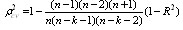 .In which n is the number of classes, k is the number of explanatory variables in the fitted model and the cross- validated R is the correlation between observed and predicted values of the dependent variable[14]. The shrinkage and contraction of the model is the positive value of λ= (
 - R2); where
 is CVPP & R2 is the coefficient of determination of the model. 1- λ is the stability of R2 of the model. Closer the value of λ to zero, the better is the prediction. The estimated CVPP related to their R2 and information on model fittings are presented in the result and discussion section. CVPP was employed as model validation test by Islam [15,16] and Islam et al.[17,18].
4. Results and Discussion
4.1. Background Characteristics of the Respondents
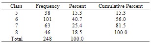
Background characteristics of the respondents are important to know the characteristics or nature of the data before performing any statistical analysis. In order to see the nature of the characteristics of data, frequency distribution and graphical representation could be very useful due to the goal of this study. For this, we perform necessary frequency tables presented below.In Table 1, it is found that 15.3% respondent are in class five, 40.7% respondent are in class six, 25.4% are in class seven and 18.5% are in class eight. Table 1. The frequency distribution of the respondents by class
 |
| |
|
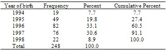
From the Table 2 it is realized that 19 respondent’s year of birth is 1994, which is 7.7%. 49 respondent’s year of birth is 1995, which is 19.8%. 82 respondent’s year of birth is 1996, which is 33.1%. 76 respondent’s year of birth is 1997, which is 30.6%. 22 respondent’s year of birth is 1998, which is 8.9%. Table 2. The distribution of the respondents by year of birth
 |
| |
|
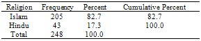
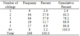
It is observed in Table 3 that 82.7% respondents are Muslim and 17.3% are Hindu. We obtain from the Table 4 that 2.4% respondent has 1 number of siblings. 37.9% respondent has 2 and 3 number of siblings. 11.7% respondent has 4 numbers of siblings. 6.9% respondent has 5 numbers of siblings and 6.9% respondent has 8 numbers of siblings.Table 3. Frequency distribution of the respondents by religion
 |
| |
|
Table 4. The frequency distribution of the respondents by number of siblings
 |
| |
|
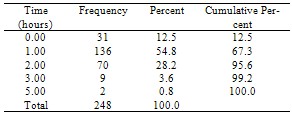
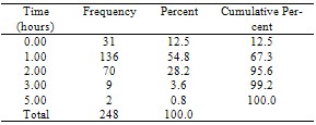
In Table 5, it is seen that 40.3% respondents are spent time with there mother less than 3 hours. 36.3% respondents spent time with there mother 3 to 7 hours. 23.4% respondents spent time with there mother more than 7 hours. We get 136 respondents are spent one hour time by playing, which is 54.8%. 70 respondents are spent 2 hour time by playing, which is 28.2%. 9 and 2 respondents are spent time 3 and 5 hour respectively, which is 3.6% and 0.8% respectively. 31 respondents are not like playing, there percentage is 12.5%.Table 5. The frequency distribution of the respondents by mother time spent
 |
| |
|
Table 6. The frequency distribution of the respondents by time spent for playing
 |
| |
|
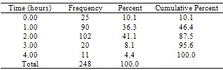
It is observed from the Table 7 that 25 respondents are not like watching TV, which is 10.1%. 90 respondents are spent one hour by watching TV, which is 36.3%. 102 respondents are spent two hours by watching TV, which is 41.1%. 20 and 11 respondents are spent 3 and 4 hours by watching TV respectively, which is 8.1% and 4.4% respectively.Table 7. The frequency distribution of the respondents by time of watching television
 |
| |
|
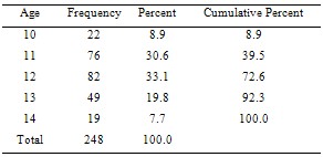
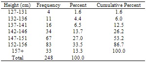
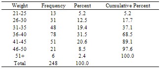
It is indicated that 22 respondent’s age is 10, which is 8.9%. 76 respondent’s age is 11, which is 30.6%. 82 respondent’s age is 12, which is 33.1%. 49 respondent’s age is 13, which is 19.8%. 19 respondent’s age is 14, which is 7.7% from the Table 8. In Table 9, we find that 127-131 cm height is 4 numbers of respondents, which is 1.6%. 132-136 cm height is 15 numbers of respondents, which is 4.4%. 137 -141 cm height is 16 respondents that is 6.5%. 142-146 cm height is 34 number of respondents, which is 13.7%. 147-151 cm height is 67 respondents which is 27%. 152-156 cm height is 83 respondents (33.5%). 157 and more cm height is 13.3%. We realize from the Table 10 that 20.6% respondent’s weight is 41-45 (in kg), which is maximum and 2.4% respondent’s weight is above 51, which is minimum. Table 8. The frequency distribution of the respondents by age
 |
| |
|
Table 9. Frequency distribution by height
 |
| |
|
Table 10. Frequency distribution of respondents by weight
 |
| |
|
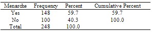
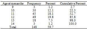
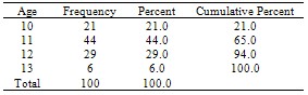
It is seen from the table that 148 (59.7%) respondents are passing their menstruation situation and 100 (40.3%) respondents are not passing this situation. We get 1 respondent’s age at menarche is 8, which is 0.4%. 2 respondent’s age at menarche is 9 that is 0.8%. 30 respondent’s age at menarche is 10 (12.1%). 45 respondent’s age at menarche is 11, which is 18.1%. 49 respondent’s age at menarche is 12 (19.8%). 18 respondent’s age at menarche is 13 (7.3%) as well as 3 respondent’s age at menarche is 14, which is 1.2%. Moreover, age distribution of non menarche students is presented in Table 13.Table 11. The frequency distribution of the respondents by menarche (yes/no)
 |
| |
|
Table 12. The frequency distribution of the respondents by age at menarche
 |
| |
|
Table 13. The frequency distribution of the age of non menarche students
 |
| |
|
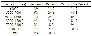
In Table 14, it is found that maximum number of respondents (29%) belong to 9000-13000 income group where as minimum number are in the age group 21000 and above.Table 14. The frequency distribution of the respondents by father income
 |
| |
|
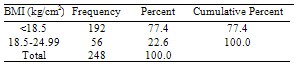
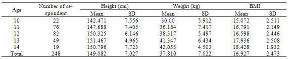
From the table we get 192 respondent’s body mass index (BMI) is below 18.5, which means that 77.4% are under weight. 56 respondent’s BMI is 18.5-24.99, which indicates 22.6% belongs to normal weight. It is observed from the Table 16 that mean height is higher in age 13, which is 151.467 and mean height is lowest in age 10 (142.471). Mean weight is highest (42.053) in age 14 and mean weight is lowest in age 10, which is 30. Mean BMI is highest in the age 14, which is 18.428 and mean BMI is lowest in age 10, which is 15.072. The mean height, weight and BMI of total respondents are 149.08, 37.180 and 16.927 respectively.Table 15. The frequency distribution of the respondents by BMI
 |
| |
|
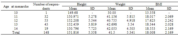
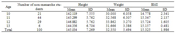
It is apprehended from the following table of menarche students that mean height is highest (152.459) in age 13 and mean height is lowest (149.68) in age 10. Mean weight is highest in age 13, which is 42.698 and mean weight is lowest in age 10, which is 30. Mean BMI is highest in age 14, which is 18.535 and mean BMI is lowest in age 10, which is 13.358. The mean height, weight and BMI of total menarche respondents are 151.816, 41.5 and 18.008 respectively.From the Table 18 it is comprehended that non-menarche students mean height is highest (146.882) in age 12 and mean height is lowest in age 10, which is 142.119. Mean weight is highest in age 12, which is 33.862 and mean weight is lowest in age 10, which is 30. Mean BMI is highest in age14 that is 15.724 and mean BMI is lowest in age 10, which is 14.778. For total non-menarche respondents, mean height, weight and BMI are 145.034, 32.350 and 15.325 respectively. Table 16. Mean values and standard deviations in height, weight and body mass index by age of total number of respondents
 |
| |
|
Table 17. Mean values and standard deviations (SD) in height, weight and BMI by age of menarche students
 |
| |
|
Table 18. Mean values and standard deviations (SD) in height, weight and body mass index by age of non-menarche students
 |
| |
|
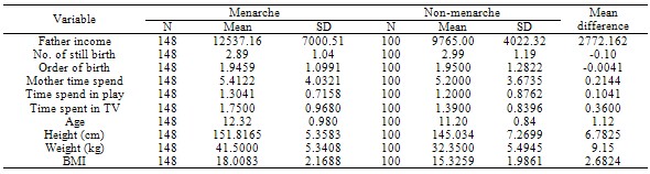
Table 19. Mean difference between menarche and non-menarche in monthly income, number of still birth, order of birth, mother time spend, time spend in play, time spend in watch TV, age, height, weight and BMI
 |
| |
|
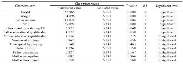
Table 20. Chi-square value and significant level of some demographic and socio-economic variables for age at menarche
 |
| |
|
The following table exhibits the mean differences in father income, number of still birth, order of birth, mother time spent, time spent in playing, time spent by watching TV, age, height, weight and body mass index in case of menarche and non-menarche respondents. The mean difference explained that father income was larger for menarche students than that of non-menarche students. Number of still birth and birth order were not significantly related to menarche and non- menarche situation. Mother time spent, time spent by playing and time spent by watching TV were larger than that of non-menarche respondents. The mean differences in age, height, weight and BMI of menarche were some what larger than those of non-menarche respondents.
4.2. Association
The contingency analysis investigated the degree or strength of association together the dependency criterion between the selected variables. Examination of association is performed by means of contingency table that is displayed in Table 20. Demographic and socio-economic variables are responsible for early menarche. We see from the table that in case of causes of early menarche for school going girl’s height, weight, father income, body mass index time spent by watching television and father educational qualification are highly significant and mother educational qualification, mother occupation, father occupation, number of siblings, order of birth, time spent by playing and mother time spent are insignificant.
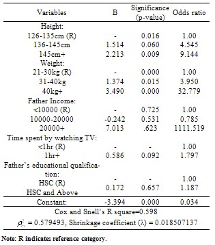
4.3. Logistic Regression Analysis
The results of logistic regression analysis are demonstrated in Table 21. The table exhibits that only three variables out of six explanatory variables are statistically significant and the rest of the variables are statistically insignificant. A brief description of the significant variables is given below:One of the most important factors for menarche is height. The estimated regression co-efficient for height group 136-145 cm and for height group 146 cm and above are 1.236 and 1.853 respectively, which means it has positive impact on menarche. The odds ratio belongs to the height groups 136-145 and 146+ cm are 3.441 and 6.378 respectively. It is indicated that 3.441 and 6.378 times higher risk of menarche than that of height group 126-135 cm. From this table it is realized that the estimated regression co-efficient for weight groups 31-40 kg and 40+ kg are 1.374 and 3.490 respectively that is positively affect on menarche. The odds ratio for the weight groups 31-40 kg and 40+ kg are 3.950 and 32.779 respectively which indicated that 3.950 and 32.779 times higher risk of menarche than that of weight groups 21-30 kg. The estimated regression coefficients for time spent by watching TV of the respondents above one hour is 0.586 which indicated that it has positive effect on menarche. The odds ratio for above one hour time spent by watching TV is 1.797. It is indicated that the risk of menarche for above one hour time spent by watching TV 1.797 times higher than that of under one hour.In the fitted logistic model, it is provided that R2=0.598,  = 0.579493, and shrinkage coefficient (λ) = 0.018507137. From these statistics, it is seen that the shrinkage coefficient is very small. Moreover, the stability of R2 of the model is more than 99%. Hence, it is concluded that the model is better fit.
Table 21. Logistic regression estimates for age at menarche with demographic and socio-economic variables
 |
| |
|
5. Conclusions
In the present study, it is found that the mean age at menarche of Bangladeshi school going girls of classes five, six, seven and eight was 12.32. This study exhibited that the father monthly income of menarche respondent’s was high than the non menarche respondent’s father monthly income. The mean difference between menarche and non-menarche respondent’s father income was 2772.622. It was displayed that the menarche students were much spent their time by watching TV and by playing and the mean difference is 0.3600 and 0.1041 respectively. The mean difference between height, weight and BMI was 6.7825, 9.15 and 2.6824 respectively, that means the taller students reached menarche earlier than the shorter girls and the heavier girls reached menarche earlier than the thinner girls and also getting larger BMI girls reached earlier than that of lower BMI girls. Height, weight, father income, BMI, time spent by watching television and father educational qualification were highly significant with the association of early menarche for school going girls. Finally, the logistic regression analysis showed that height, weight and time spent by watching TV of the respondents had positive effects on age at menarche.
References
| [1] | Kelsey, J. (1993). Breast cancer. Epidemiologic Reviews., 15: 1-263. |
| [2] | Copper, G., Ephross, S., Weinberg, C., Baird, D. and Sandler, D. (1998). Menstrual and reproductive risk factors for ischemic heart disease. Epidemiology., 10: 255-259. |
| [3] | Rees, M (1995). The age at menarche. ORGYN., 4:2-4. |
| [4] | Riley, A.P., Huffman, S.L. and Chowdhury, A.k. (1989). Age at menarche and postmenarcheal growth in rural Bangladeshi females. Ann Hum Biol., 16: 347-359. |
| [5] | Wyshak, G. and Frisch, R. (1982). Evidence for a secular trend in age at menarche, New England Journal of Medicine, 306: 1033-1035. |
| [6] | Roberts, D. and Dann, T. (1975). A 12 year study of menarcheal age, British Journal Of Preventive and Social Medicine, 29: 31-39. |
| [7] | Hauspie, R., Vereauteren, M. and Susanne, C. (1997). Seqular changes in growth and maturation: an update. Acta Padiatrica., 423:20-27. |
| [8] | Chowdhury, A.K, Huffman, S.L, and Curlin, G.T. (1977). Malnutririon menarche and marriage in rural . 24: 316-325. |
| [9] | Haq, M.N. (1984). Age at menarche and the related issue: a pilot study on urban School girls. J Youth Adolesc., 13:559-567. |
| [10] | Ogata (1979). Age at menarche and marriage in women. J Trop Med Hyg., 82: 68-74. |
| [11] | Cox, D. R. (1958). The regression analysis of binary sequences (with discussion), J.R. Statist. Soc., B20, pp.215-242. |
| [12] | Cox, D. R. (1970). The analysis of binary data, : , Chapman and Hall Ltd. |
| [13] | Fox, J. (1984). Linear statistical models and related methods, Wiley and Sons, . |
| [14] | Stevens, J. (1996). Applied Multivariate Statistics for the Social Sciences, Third Edition, Lawrence Erlbaum Associates, Inc., Publishers, . |
| [15] | Islam, Rafiqul (2003). Modeling of Demographic Parameters of -An Empirical Forecasting, Unpublished Ph.D. Thesis, . |
| [16] | Islam, Rafiqul. (2005). Construction of Female Life Table from Male Widowed Information of , J. of Statistics, Vol. 21(3), Page 275-284. |
| [17] | Islam, Rafiqul, Islam, Nurul, Ali, Md. Ayub and Golam (2003). Construction of Male Life Table from Female Widowed Information of Bangladesh, International J. of Statistical Sciences, Vol. 2, Dept. of Statistics, University of Rajshahi, Bangladesh, Page 69-82. |
| [18] | Islam, Rafiqul, Islam, Nurul, Ali, M. Korban & Mondal, Md. Nazrul Islam (2005). Indirect Estimation and Mathematical Modeling of Some Demographic Parameters of , The Oriental Anthropologist, Vol. 5(2), Page 163 - 171. |
 Abstract
 Reference
 Full-Text PDF
 Full-Text HTML