-
Paper Information
- Paper Submission
-
Journal Information
- About This Journal
- Editorial Board
- Current Issue
- Archive
- Author Guidelines
- Contact Us
American Journal of Intelligent Systems
p-ISSN: 2165-8978 e-ISSN: 2165-8994
2022; 12(2): 51-58
doi:10.5923/j.ajis.20221202.02
Received: Jan. 17, 2021; Accepted: Jul. 20, 2022; Published: Jul. 29, 2022

Comparative Study of Adaptive Neuro-Fuzzy Inference System and Artificial Neural Network for Online Harmonic Mitigation
 Abstract
 Reference
 Full-Text PDF
 Full-text HTML
Adeyemo I. A.1, Ojo J. A.1, Ola O. M.2, Babajide D. O.1
1Electronic & Electrical Engineering Dept, Ladoke Akintola University of Technology, Ogbomoso, Oyo State, Nigeria
2Works & Services Unit, Bowen University, Iwo, Osun State, Nigeria
Correspondence to: Adeyemo I. A., Electronic & Electrical Engineering Dept, Ladoke Akintola University of Technology, Ogbomoso, Oyo State, Nigeria.
| Email: |  |
Copyright © 2022 The Author(s). Published by Scientific & Academic Publishing.
This work is licensed under the Creative Commons Attribution International License (CC BY).
http://creativecommons.org/licenses/by/4.0/

Solving the transcendental nonlinear equations characterizing harmonics in multilevel converters in real time is presently infeasible due to heavy computational burden in terms of memory and computational time. To overcome this problem, artificial intelligence based predictive models are used. This paper presents a comparative study and performance evaluation of artificial neural network (ANN) and adaptive neuro-fuzzy inference system (ANFIS), which are the leading predictive models for modeling nonlinear systems such as the relationship between the modulation index and switching angles in multilevel converters. The performance of both ANN and ANFIS are evaluated in terms of accuracy, convergence behaviour as well as learning and generalization capabilities using coefficient of determination (R2), root mean square error (RMSE) and mean absolute error (MAE) as the performance evaluation metrics. The results of simulations performed in MATLAB/SIMULINK environment are also presented to validate the predictions made by the models.
Keywords: ANN, ANFIS, Multilevel inverter, Selective Harmonics Elimination (SHE), Newton Raphson method
Cite this paper: Adeyemo I. A., Ojo J. A., Ola O. M., Babajide D. O., Comparative Study of Adaptive Neuro-Fuzzy Inference System and Artificial Neural Network for Online Harmonic Mitigation, American Journal of Intelligent Systems, Vol. 12 No. 2, 2022, pp. 51-58. doi: 10.5923/j.ajis.20221202.02.
Article Outline
1. Introduction
- In recent years, global power demand has increased substantially while the expansion of the traditional power systems has been severely limited by rapid depletion of fossil fuel, energy crisis and environmental restrictions such as Clean Air Act of 1970 and Kyoto protocol of 1997. This has resulted into dramatic changes in the modern electric power production in terms of both physical and control infrastructures with power electronics playing a key role. The electric power industry is gradually witnessing a paradigm shift from the traditional power system to distributed power system. In the traditional power systems, a relatively few but large power generation plants located at adequate geographical places produce bulk of the power, which is then transmitted over mostly high voltage ac grid to consumers located a long distance away [1]. However, in the emerging modern power systems, there are many diverse, dispersed and distributed generation (DG) plants with the transmission of electricity over smart grid comprising of both alternating current (AC) and direct current (DC) transmission lines. High-voltage, direct current (HVDC) electric power transmission system facilitates transfer of power between unsynchronized AC transmission systems such as grid systems operating at different frequencies. Distributed power system includes arrays of solar photovoltaic panels, wind farms, hydroelectric, biomass and tidal power plants. Among distributed power generation schemes, wind farms and solar technology are the most promising schemes, even envisaged as competing with the traditional fossil-fuelled thermal power plants in the near future [2]. Consequently, the share of renewable energy sources in the overall global generation mix is gradually increasing, and it is expected that renewable energy sources will turn out to be an important part of the global energy policy. However, renewable energy sources have highly variable daily and seasonal patterns, and consumer power demand requirements are also extremely variable in nature. Power electronic converters have been recognised as the interface for integrating distributed generators with the utility grid. DC- to - AC power electronic converters are known as inverters. The function of a voltage source inverter (VSI) is to synthesize an output AC voltage of desired magnitude and frequency from a slowly varying DC input voltage [3]. A multilevel inverter is a power electronic converter that synthesizes a desired AC output voltage from several levels of DC input voltages such that a staircase voltage waveform that is nearly sinusoidal is obtained with minimum harmonic distortion. Due to their spectral performance and ability to attain a higher voltage without transformer, multilevel inverters have been drawing increasing attention in recent years, especially in the distributed power generation area, because several batteries, fuel cells, solar cells, or rectified wind turbines or microturbines can be connected through a multilevel inverter to feed local loads or interconnect to the AC grid without voltage balancing problems [1]. In addition, multilevel inverters have a lower electro-magnetic interference (EMI), lower switching frequency with the consequent reduction in the switching losses. Multilevel inverters are also widely used in high-voltage and high-power applications such as high voltage direct current (HVDC) transmission, flexible AC transmission system (FACTS) and adjustable speed drives (ASD) etc. Several pulse width modulation (PWM) methods have been developed for the control of multilevel inverters among which are space vector PWM (SVM), sinusoidal PWM (SPWM), selective harmonic elimination pulse width modulation (SHEPWM) etc. The control of multilevel inverters using SHEPWM technique at fundamental switching frequency is prevalent in power industry. This can be attributed to its direct control of harmonics and synthesis of high-quality output voltage. However, the deployment of SHEPWM technique for real time applications is presently infeasible due to the heavy computational cost involved in finding the solution of the nonlinear and transcendental equations known as selective harmonic elimination (SHE) equations that contain trigonometric terms. The solution of SHE equations yields solution sets at various modulation indices that ensure the synthesis of the desired fundamental output voltage as well as the elimination of the selected lower order harmonics. The traditional methods used for solving this kind of nonlinear optimization problems include derivative-dependent method like Newton Raphson method [4], which diverges if the arbitrarily chosen initial values are not close enough to the roots. It also risks being trapped at a local optimum and fails to give best solution. Chiasson et al [5,6] proposed a method based on Elimination theory using resultants of polynomials to determine the solutions of the SHE equations. A difficulty with this approach is that as the number of levels increases, the order of the polynomials becomes very high, thereby making the computations of solutions of these polynomial equations very complex. Another approach uses Walsh functions [7,8] where solving linear equations, instead of non-linear transcendental equations, optimizes the switching angle. The method results in a set of algebraic matrix equations and the calculation of the optimal switching angles is a complex and time-consuming operation. Evolutionary algorithms like ant colony optimization (ACO) [9], particle swarm optimization (PSO) [10,11] and Genetic Algorithm (GA) [12,13] are derivative free and are successful in locating the optimal solution, but they are usually slow in convergence and require much computing time.All the aforementioned methods suffer from excessive computational time spent on solving the SHE equations that characterize the optimal switching angles; hence real-time computation of switching angles in multilevel inverter is currently infeasible and the angles are computed offline. A method that is currently in use for the real time applications of SHEPWM is called programmed SHEPWM. In this approach, the offline pre-computed switching angles for the required values of modulation index are stored as look-up tables in the memory of microprocessor-based modulator. The major drawback of this approach is that a large memory is required to store the look-up tables. With the increasing use of power conditioning systems in online applications such as electric vehicle (EV), adjustable speed drive (ASD), static synchronous compensator (STATCOM), dynamic voltage restorer (DVR) and other FACTS devices, real time solution of SHE equations has continued to garner interest in order to harness the merits of SHEPWM technique. The advances made in predictive modeling using mathematical statistics has enabled researchers to overcome the difficulty involved in solving SHE problem with the deployment of artificial intelligence (AI). Real time implementation of the predictive models has also been aided by the advancement made in digital signal processing (DSP) as well as the proliferation of high-power and high-speed semiconductor devices. A major advantage of the predictive models over programmed SHEPWM is that they do not suffer from memory constraint since they do not require look-up tables to save the precalculated values. This is due to their ability to interpolate and extrapolate once they are properly trained with the offline results previously computed with either analytical or evolutionary algorithm. From the literature, the leading predictive models for the real time generation of solution sets for the SHEPWM controlled multilevel inverters are artificial neural network (ANN) [14] and adaptive neuro-fuzzy inference system (ANFIS) [15]. In this paper, both ANN and ANFIS are deployed for the input-output mapping of modulation index and optimal switching angles in cascaded H-bridge multilevel inverter. In both cases, Newton Raphson iterative method serves as the teacher that generates the initial dataset used for the training purpose.
2. Literature Review
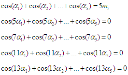
- A. CASCADED H-BRIDGE MULTILEVEL INVERTERS AND SHE TECHNIQUECascaded H-bridge multilevel inverters (CMLI) are created by series connection of two or more H-bridge converters, each supplied by an isolated source on the DC side and series-connected on the AC side. Each H-bridge converter can generate three different voltage levels: +Vdc, 0, and -Vdc by connecting the DC source to the AC output by different combinations of the four switches S1, S2, S3, and S4 shown in the Figure 1. To obtain +Vdc, switches S1 and S4 are turned on, whereas –Vdc can be obtained by turning on switches S2 and S3. By turning on S1 and S2, or S3 and S4, the output voltage is zero. Each converter generates a square wave voltage waveform with different duty cycles. The output voltage is the summation of all voltages from the cascaded H-bridge cells [16]. The total number of output voltage levels in a cascaded H-Bridge inverter is defined by n =2s +1, where s is the number H-bridges per phase connected in cascade. The structure of a single-phase cascaded H-bridge multilevel inverter is shown in Figure 1 and the output voltage waveform of a single-phase 11-level CHB inverter is shown in Figure 2.
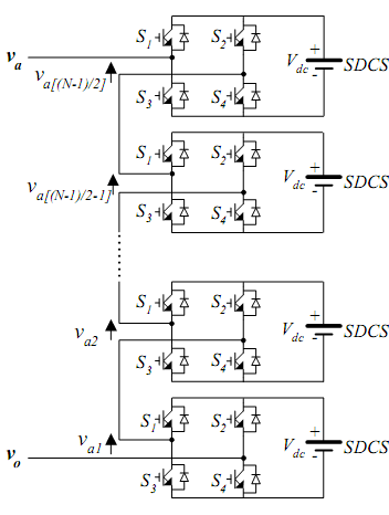 | Figure 1. Single-phase structure of an N-level CHB inverter |
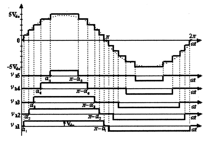 | Figure 2. Output voltage waveform of a single-phase 11-level CHB inverter |
 | (1) |
 | (2) |
 | (3) |
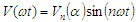
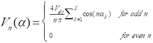
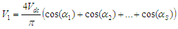
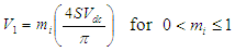
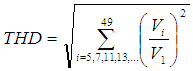
 Where S is the number of SHE equations or degrees of freedom and n is the harmonic order. Generally, for S number of degrees of freedom, one degree of freedom is used for controlling the magnitude of the desired fundamental output voltage V1 and the remaining (S-1) degrees of freedom are used to eliminate the selected lower order harmonics that are dominant in the total harmonic distortion (THD). From equation (3), the expression for fundamental output voltage is given by
 | (4) |
 | (5) |
 | (6) |
 | (7) |
 | (8) |
 | (9) |
 | (10) |
 and bias (b) of the network [18].
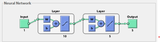 | Figure 3. Typical feedforward ANN |
 are normally continuous variable with n being the number of inputs to the neuron. Each of the inputs
  is multiplied by an associated adjustable scalar weight
  , which can be positive or negative corresponding to acceleration or inhibition of the flow of signals. Neurons belonging to adjacent layers are fully connected and the activation function of the neurons is generally sigmoid, inverse tan, hyperbolic, Gaussian or linear.
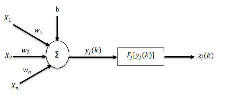 | Figure 4. Structure of a single artificial neuron |
 | (11) |
 | (12) |
 = i-th input signal of the neuron
 = weight associated with the i-th input signalb = adjustable bias associated with the neuron
 = weighted response (summing junction) of the j-th neuron with respect to instant k.
 = activation function of the j-th neuron
 = output signal of the j-th neuron with respect to the instant k.The adjustment process of the network weights
  associated with the j-th output neuron is done from computation of error signal with respect to the k-th iteration. This error signal is given by the following equation:
  | (13) |
 is the desired output at the j-th output neuron.In the back propagation algorithm, the performance criterion is based on the mean-squared error function, which is defined as the summation of all squared errors produced by the output neurons of the network with respect to k-th iteration yields
  | (14) |
 so that for each data set,
 | (15) |
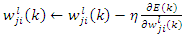 | (16) |
 is the weight connecting the j-th neuron of the l-layer to the i-th neuron of the (l-1) layer, and η is a constant that determines the learning rate of the back-propagation algorithm. The weights belonging to the hidden layer of the network are adjusted in similar manner.C. ADAPTIVE NEURO-FUZZY INFERENCE SYSTEM (ANFIS)Adaptive neuro-fuzzy inference system (ANFIS) can simply be described as a fuzzy inference system (FIS) trained by adaptive artificial neural network (ANN) [19]. While the strength of ANN lies in its non-linear input-output mapping ability by learning from knowledge base without knowing the underlying mathematical relationship, however, it lacks heuristic sense and it works like a black box. On the other hand, the strength of rule-based fuzzy logic (FL) lies in its capability to transform heuristic and linguistic terms into numerical values and vice versa through fuzzy rules and membership function. However, FL is plagued by the difficulty involved in finding the accurate fuzzy rules and membership functions, which are heavily dependent on the prior knowledge of the system. By combining ANN with FL, ANFIS uses the adaptive data-based training process of ANN to tune the parameters of the fuzzy inference system. Thus, ANFIS combines the adaptive learning capability of ANN with the robustness and imprecise or distorted data usage capability of FL. Figure 5 shows the architecture of a five-layer ANFIS with two inputs and a single output. The nodes of layers one and four are adaptive nodes, which are represented by squares while the nodes of layers two, three and five are fixed nodes that are represented by circles.
 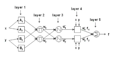 | Figure 5. ANFIS structure for two input variables and five layers |
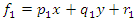 Rule 2: if x is A2 and y is B2, then
 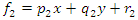 Where x and y are the crisp inputs, Ai and Bi are the linguistic variables associated with the node function. The output of each node in every layer can be denoted by
  where i is the node number and l is the prevailing layer number. The first layer is called the fuzzification layer. The parameters in this layer are called premise parameters, and every node in this layer is an adaptive node. In this layer, there is transformation of crisp input variables into fuzzy variables. The crisp input variables are assigned membership functions, which determines their degree of membership of a fuzzy set. The outputs of the fuzzification layer are the membership grade of the crisp inputs, and they are expressed as follows:For x input to node i,
  For y input to node i,
  Where
Where  and
and  are membership functions that determine the degree to which the given x and y satisfy the quantifiers Ai and Bi.The second layer is called antecedent rule layer. The degree of fulfilment (DOF) is determined for each rule in this layer. The firing strength for each rule, which qualifies the extent to which any input data belong to that rule is calculated. Every node in this layer is a fixed node, whose output represents the firing strength of a rule, and the firing strength represents the IF conditions to set the rules. The output of this layer is the algebraic product of the input signals given as:
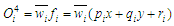
 | (17) |
 | (18) |
 | (19) |
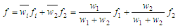
 is the output of the third layer and
  is the parameter set of node i. These parameters are referred to as consequent parameters. The last layer is the summation layer. It contains a single fixed node labeled
  which computes the overall output by summing all the incoming signals.
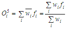 | (20) |
 | (21) |
3. Implementation
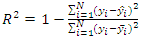
- The first step in ANN modeling is the choice of topology of the network. Multilayer feedforward ANN topology with back propagation of error was chosen to develop the switching angles prediction model that maps the input data (modulation index) to the output data (switching angles). Using different transfer functions, several ANN models with only one neuron in the input layer, five neurons in the output layer and different numbers of neurons in the hidden layer were developed, trained and tested. The ANN model chosen as optimal comprises of an input layer with only one neuron, a hidden layer with thirty neurons, scalar weights, biases and sigmoid transfer function, and an output layer with five neurons, scalar weights, biases and linear transfer function. The network training was performed with Fletcher-Reeves variant of back propagation algorithm using the data generated by Newton Raphson. For ANFIS modeling, eight (8) ANFIS models with the same number of membership function (NMF), different types of input membership function (IMF) and output membership function (IMF) were constructed and evaluated in order to select the best-fit fuzzy model.For the implementation of both ANN and ANFIS models, the original dataset generated by Newton Raphson method was randomly divided into three subsets: training (70%), testing (15%) and validation (15%). The first subset is for training and network is adjusted to its error. The second subset is used to measure network generalization and to halt training when generalization stops improving. The third subset provides an independent measure of network performance during and after training. The maximum number of epochs in both models is 500.Performance Evaluation MetricsThe coefficient of determination (R2), Root Mean Square Error (RMSE), and Mean Absolute Error (MAE) are used to evaluate the performance of the prediction models in regression analysis.The coefficient of determination (R2) is a statistical measure in linear regression model that determines the proportion of the variance in the dependent variable that is predictable from the independent variable(s). It is a scale-free score, and its value is less than one.
 | (22) |
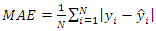 | (23) |
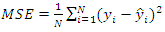 | (24) |
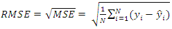 | (25) |
 is the predicted value of y,
  is the average value of y and N is the number of observations available for analysis.
4. Results and Evaluation of the Prediction Models
- A personal computer (2.11 GHz Intel Core i5 processor with 8.00 GB Random Access Memory and 930 GB Hard disk drive) running MATLAB R2018a on Windows 10 was used to carry out the calculations. Several ANN models with different topologies were trained, tested and evaluated to select the best network topology. The values of
 , MAE and RMSE for different ANN topologies are presented in Table 1.
|
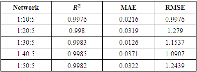
 and RMSE compared with 1:50:5 while topology 1:30:5 has the least value of MAE which indicate that performance does not necessarily improved with increasing number of neurons in the hidden layer. Topology 1:40:5 has the highest value of
  but its value of MAE is more than twice the value obtained for topology 1:30:5. Comparative analysis of the values of
  , MAE and RMSE for different ANN topologies presented in Table 1 shows that topology 1:30:5 is the optimal model.Different types of input membership functions (IMF) and output membership function (OMF) were evaluated for ANFIS model. The optimal number of membership function (NMF) was found to be 20. The values of
  , MAE and RMSE for different ANFIS models are presented in Table 2.
|
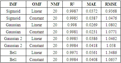
 and the least value of RMSE (0.9368).With the optimal topology of ANN model and IMF/OMF of ANFIS model chosen to be 1:30:5 and Sigmoid/Linear, respectively. The values of
  , MAE and RMSE are (0.9983, 0.0126, 1.1537) and (0.9987, 0.0372, 0.9368) for the chosen ANN model and ANFIS model, respectively. Shown in Figure 6 are the plots of switching angles versus modulation index for NR computed, ANN predicted and ANFIS predicted solution sets, respectively.
 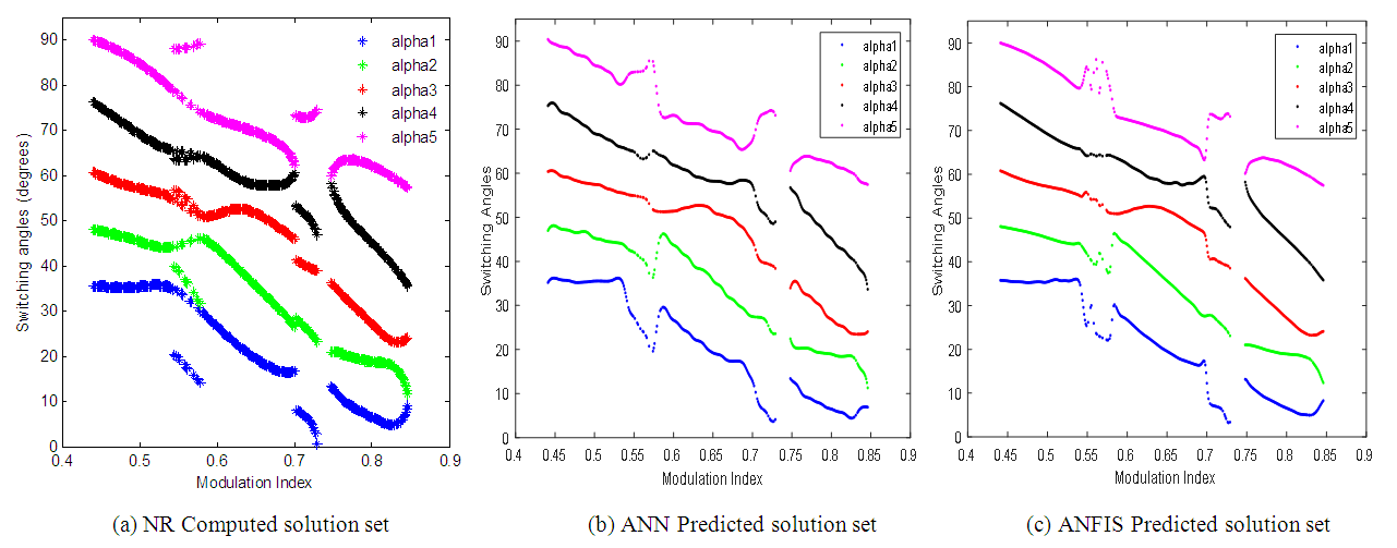 | Figure 6. Plots of switching angles versus modulation index for (a) NR (b) ANN and (c) ANFIS models |
|
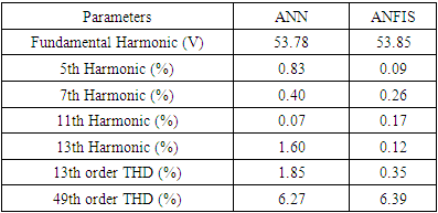
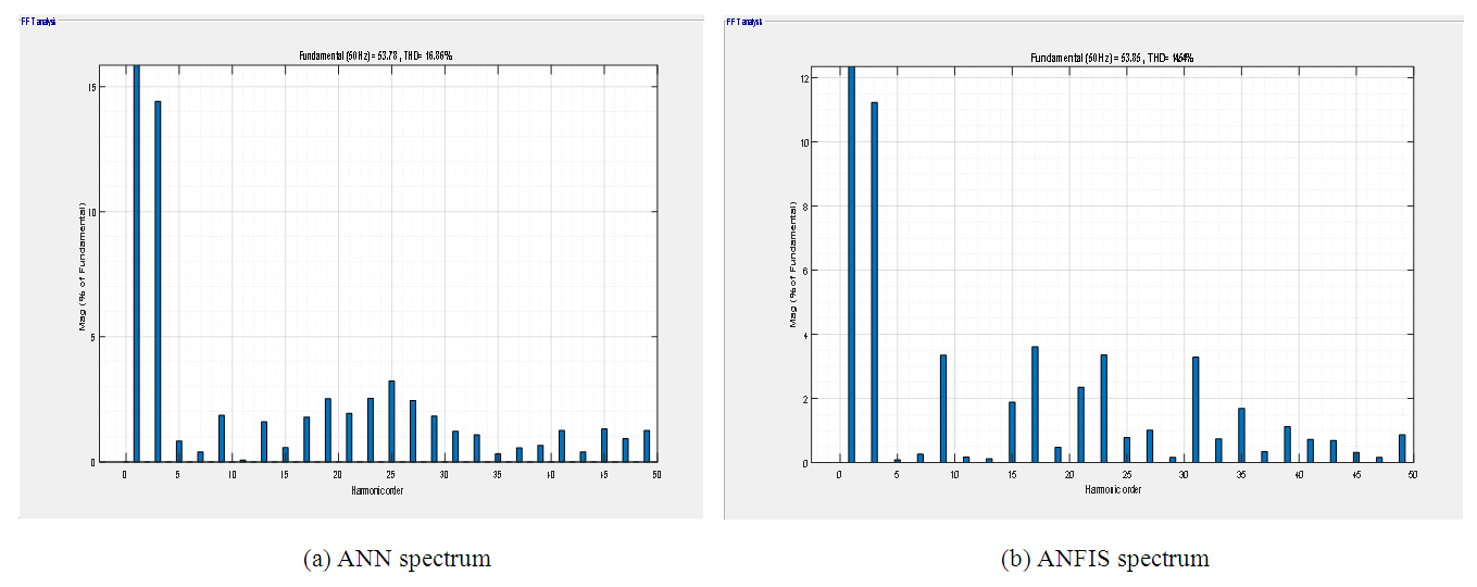 | Figure 7. Harmonic spectra of (a) ANN and (b) ANFIS solution sets at the same modulation index of 0.703 |
5. Conclusions
- Comparative study of ANN and ANFIS models for the real time computation of switching angles in an 11-level inverter is presented in this study. Using dataset previously computed offline with Newton Raphson iterative method, both models were trained and simulated in MATLAB for real time generation of optimal switching angles. The comparative study of the statistical values of
 , MAE and RMSE for ANN and ANFIS model shows that ANN outperform ANFIS in term of MAE while ANFIS have better values of
  and RMSE. Both models demonstrated good generalization capability for the generation of accurate solution sets for SHEPWM controlled multilevel inverters in real time. However, simulation results show that ANN is more efficient for THD minimization while ANFIS is more suitable for the selected lower order harmonics elimination. The findings of this study will aid other researchers in the area of artificial intelligence (AI) based forecasting techniques in their choice of the appropriate predictive model. Future research on the findings of this study could be done to establish ANN and ANFIS as viable alternatives to time series analysis or linear regression.